-
Paper Information
- Next Paper
- Paper Submission
-
Journal Information
- About This Journal
- Editorial Board
- Current Issue
- Archive
- Author Guidelines
- Contact Us
American Journal of Operational Research
p-ISSN: 2324-6537 e-ISSN: 2324-6545
2020; 10(2): 23-29
doi:10.5923/j.ajor.20201002.01
Received: Jul. 21, 2020; Accepted: Aug. 27, 2020; Published: Sep. 15, 2020

Time Series Analysis of KSE-100 Using Box- Jenkin’s Methodology
 Abstract
 Reference
 Full-Text PDF
 Full-text HTML
M. Haseeb Khan, Nadia Mushtaq
Department of Statistics, Forman Christian College University, Lahore, Pakistan
Correspondence to: Nadia Mushtaq, Department of Statistics, Forman Christian College University, Lahore, Pakistan.
| Email: |  |
Copyright © 2020 The Author(s). Published by Scientific & Academic Publishing.
This work is licensed under the Creative Commons Attribution International License (CC BY).
http://creativecommons.org/licenses/by/4.0/

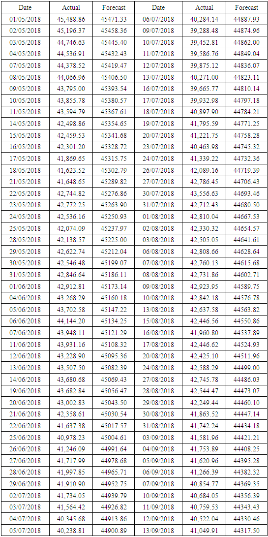
The stock market is one of the biggest sectors for generating capital for both investor and company as well as for the government and it plays a vital role for the economic progress of any country. The most reliable way to calculate the stock market performance is to check its indices. We are taking KSE-100 Index of Pakistan Stock Exchange (PSX) as it is one of the best performing Index with companies having large capitalization to analyze and forecast its values based on the data of 250 days from 1st May 2017 – 30th April 2018 to the next 90 days by using Box-Jenkins methodology. We also compare the forecast values with actual values, and we can observe that the fits behave more like the actuals.
Keywords: Box-Jenkin’s Methodology, Forecast, KSE-100 Index
Cite this paper: M. Haseeb Khan, Nadia Mushtaq, Time Series Analysis of KSE-100 Using Box- Jenkin’s Methodology, American Journal of Operational Research, Vol. 10 No. 2, 2020, pp. 23-29. doi: 10.5923/j.ajor.20201002.01.
Article Outline
1. Introduction
- The stock market is a platform which deals with the trading of securities through various physical and electronic means. It allows investors to buy shares of ownership in a company which means he is entitled in profit and loss of a company and because of this it runs on the principle of market economy. The main purpose for which the investors buy shares of the companies is to sell them at a higher price to gain profit on their investment but not everyone succeeds in gaining return on their investment because of the constant fluctuation in the prices of stocks. To keep themselves on safer side, the investors analyze the market on the basis of its indices. A stock index is said to be measurement of the section of stock market which measures the change of stock prices of its components. In this paper, we are going to talk about the KSE-100 Index of PSX. The index was launched in Nov 1991. It is taken as an Index having companies with large capitalization. It consists of 100 companies and is the most generally accepted measure with about 90% market capitalization of the whole PSX. Everyone wants to predict the future in order to secure his investments. However, the future is always uncertain but the investor always wants to invest the spare money in order to obtain lucrative results. The fluctuation in the stock market is due to many reasons, some which are really hard to predict but whatever it maybe but it indicates the direction of the economy. Higher the stock market capitalization, higher the company’s valuation and in return higher the country’s economy. There are mainly two methods for the time series forecast. One method is to take explanatory variables in regression analysis by taking factors that are responsible to fluctuate the stock market. It has a drawback. Many factors are not easy to understand or to measure and in some cases the required data is not available. However, there is also another method in which we predict the future value based on the past ones. One such model which we are using is and Autoregressive Integrated Moving Average (ARIMA) model in case of non-stationarity. Non-stationarity is defined by Gujarati & Porter (2004) as the one that hasn’t a constant long-run mean and a time-invariant covariance. In ARIMA model, time series is forecasted on the basis of its previous values and previous residuals value. We are following the Box-Jenkin’s methodology to do this research. Box and Jenkins published this methodology in their renowned book “Time Series Analysis: Forecasting and Control”. Box & Jenkins (1970) helps us to identify importance of lagged value and residuals of a variable in predicting its future value. The objective of our study is to forecast the values of KSE-100 based on the data from 1st May 2017 – 30th April 2018 for the next 90 days and also compare the forecast values with actual values so that we can observe that either the fits behave more like the actuals.
2. Literature Review
- Forecasting is an interesting area of research for the researchers and it will continue to fascinate to better the current predictive models. The reason is that everyone can make an investment in the light of decisions and ability to plan and develop effective strategy about their daily and future financial desires. Pai, P. et al. (2005) said that stock price forecasting is one of most troublesome assignment to accomplish in financial forecasting due to complex nature of stock market. Stock market predictors always try to develop successful techniques for forecasting index value of prices. The fundamental point is to acquire high profit utilizing best trading strategies and a successful stock market prediction to achieve best result and also to minimize inaccurate forecast stock price. The objective of investors is to make any forecasting strategy that could help them in easy benefitting and limiting investment risk from the stock market. Wang, J.J. et al. (2012) said that the prediction should be possible from two perspectives: statistical and artificial intelligence techniques.Chi. S.C. et al. (1999) told us that there are two analytical models to anticipate the stock market, namely, fundamental analysis and technical analysis. Fundamental analysis deals with economic analysis, industry analysis and company analysis. Technical analysis ensures us with predicting future price based on the past market data. Time series model is a dynamic research field which has pulled in considerations of analysts group over last couple of decades. Raicharoen, T. et al. (2003) said that the fundamental point of time arrangement demonstrating is to precisely gather and thoroughly ponder the past perceptions of a period arrangement to build up a proper model which depicts the inalienable structure of the arrangement. This model is then used to create future esteems for the arrangement, i.e. to make estimates. Zhang, G.P. (2007) described that time series models determine along these lines can be named as the demonstration of foreseeing the future by comprehension the past. Because of the crucial significance of time series models is to determine in various fields, for example, business, financial aspects, economics, science and engineering, etc., high care ought to be taken to fit a satisfactory time series model to the required arrangement. Tong, H. (1983) describes that an effective time series analysis relies upon a proper model fitting. A huge amount of work has been done by analysts over various years for the advancement of capable models to enhance the forecasting accuracy. Accordingly, different important time series forecasting models have been made. Raicharoen, T. et al. (2003) elaborated that time series forecasting thus can be called as the demonstration of foreseeing the future by understanding the past.Bagnall, A.J. et al. (2004) emphasized that forecasting of stock prices has attracted attention from the research community. Time series analysis covers an extensive number of forecasting methods. Researchers have built up various modifications to the basic ARIMA model and found impressive achievements in these methods. The modifications incorporate clustering time series from ARMA models with clipped data.Ali, A. et al. (2011), used ARIMA models to forecast stock market performance of the Oil and Gas Companies in Pakistan.Mondal, P. et al. (2014) applied ARIMA model on 56 stocks of India from different sectors in order to forecast their future returns. Their research concluded with being 85% successful forecasts.Banerjee, D. (2014) utilized ARIMA model to forecast Indian stock market index. He concluded with the result that the short run prediction power is most suitable for the model in order to take best results.Time series analysis is the approach of prediction that focuses on the previous behaviour of dependent variable. Time series models give another approach to analyze and forecast future developments based on previous behaviour of the objective. Fang, J. et al. (2003) concluded that time-series forecasting has been usually performed using statistical-based methods, for example, the linear autoregressive (AR) models because of their flexibility to model many stationary processes. These include the ARMA (autoregressive moving average) model. Methods such as the linear autoregressive integrated moving average (ARIMA) is based on the evolution of the increments are used at times to remove or reduce first order non-stationarity. Hipel, K.W. et al. (1994) concluded that the concept of stationarity can be seen as a form of statistical equilibrium. The properties of mean and variance of a stationary process do not rely on time. There is a greater possibility that the time series will not be stationary if there is a greater historical observations data whereas for short time span we usually use differencing or transformation in our model to make it stationary.
3. Box-Jenkins Methodology
- The model consists of three main approaches:
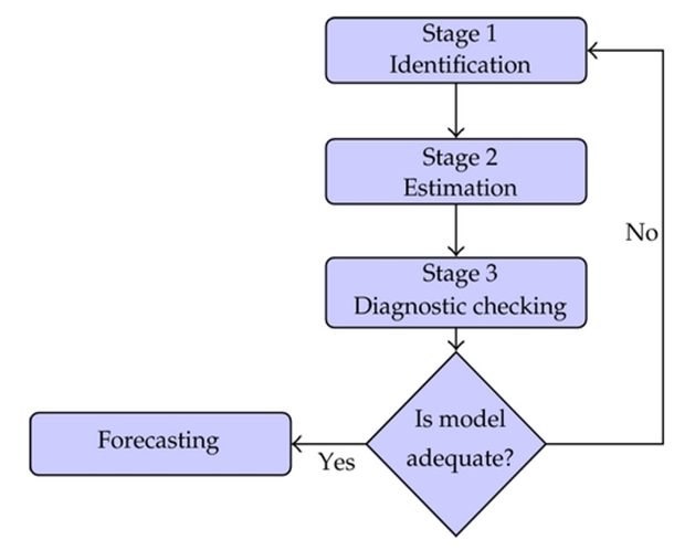 | Figure 1. Stages of Box-Jenkins Methodology |
|
4. Research Methodology
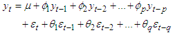
- In the beginning, we will apply ARMA model if we get the stationary data. Stationarity is defined by Gujarati & Porter (2004) as the one that has a constant long-run mean and a time-invariant covariance. If the data is non-stationary then we will apply ARIMA model.Autoregressive Moving Average (ARMA) model gives the explanation of a stationary process in terms of two polynomials, one for the autoregressive (p) and the second for the moving average (q). We express the ARMA(p,q) in mathematical form given as:
 | (1) |
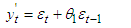
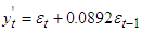
 yt represents the variable we are trying to predict yt-1, yt-2,…yt-p are the previous or lagged values of that variable that are also called the autoregressive terms εt is the disturbance or error term, εt-1, εt-2,…, εt-q are the previous or lagged values of the error term that are also known as the moving averages φ1, φ2 ,…, φp are the coefficients of autoregressive terms θ1, θ2, … , θp are the coefficients of the moving average regressorsAutoregressive Integrated Moving Average (ARIMA) model is a conception of an autoregressive moving average (ARMA) model. Both of these models are applied to time series data for the better understanding of the data or to forecast future values in the series forecasting. These are mostly applied where the data is of non-stationary to make it stationary. It is composed of two parts• an integrated (I) component (d) that represents the amount of differencing to be applied on the time series to make it stationary• the autoregressive moving average (ARMA) modelWe express the ARIMA (p,d,q) in mathematical form given as:
  | (2) |
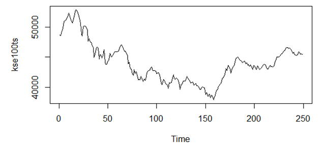 | Figure 2. Time Series Plot of KSE-100 (1st May, 2017- 30th April, 2018) |
|
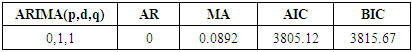
 | (3) |
 | (4) |
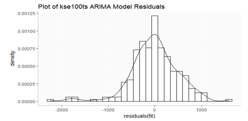 | Figure 3. Histogram of residuals of ARIMA (0,1,1) model of KSE-100 |
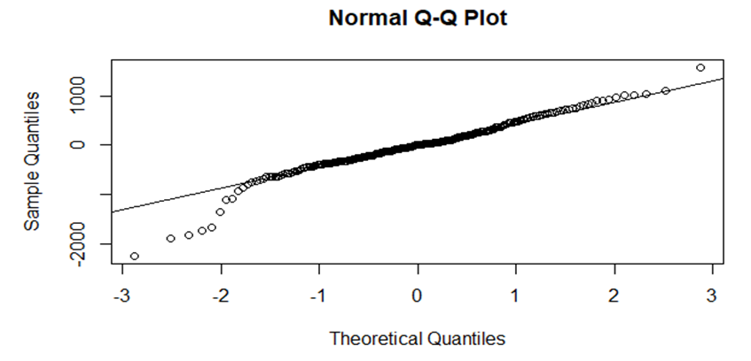 | Figure 4. Normal QQ Plot of residuals of ARIMA(0,1,1) model of KSE-100 |
 | (5) |
|
|
|
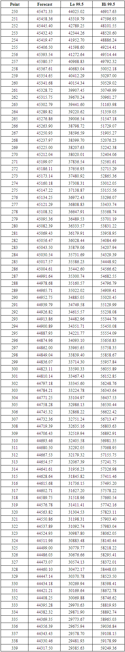
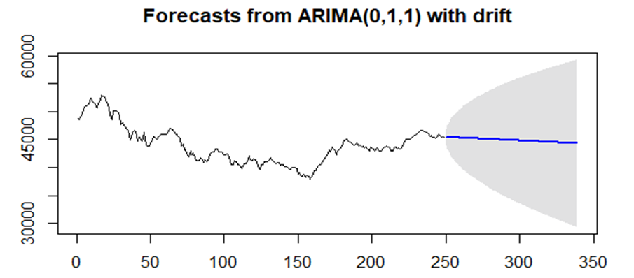 | Figure 5. Forecast plot of KSE-100 by ARIMA (0,1,1) model |
5. Conclusions
- In this work, we have analyzed the indices of PSX during 1st May 2017 – 30th April 2018. Here, we have index namely KSE-100. By looking at the forecasting results and graphs of KSE-100, we may conclude that in the future, the stock market is going to become bearish with the constant declination in the trend at least for next 90 days. We also compared the forecast values with actual values, and we can observe that the fits behave more like the actuals.