Patrick R. McMullen
Wake Forest University, Winston-Salem, NC 27106, USA
Correspondence to: Patrick R. McMullen, Wake Forest University, Winston-Salem, NC 27106, USA.
| Email: |  |
Copyright © 2019 The Author(s). Published by Scientific & Academic Publishing.
This work is licensed under the Creative Commons Attribution International License (CC BY).
http://creativecommons.org/licenses/by/4.0/

Abstract
This research presents a simulation-based approach to establishing stations for an urban bike-sharing system. Movements of bicycles from one station to another are simulated via a Markov process. During the simulation, some stations will lose bicycles, while other stations will gain bicycles. This simulation process is tantamount to the transient phase of a Markov process. Sparsely-used stations are closed, resulting in increased system utilization. The simulation is applied to several test problems. Experimentation shows 86.53% average system utilization, with a standard deviation of 6.81%. It was also discovered that more bikes in the system requires more simulation time, along with more sensitivity to minimum utilization thresholds.
Keywords:
Simulation, Markov, Optimization, Utilization
Cite this paper: Patrick R. McMullen, A Markov Simulation Approach to Balancing Bike-Sharing Systems, American Journal of Operational Research, Vol. 9 No. 1, 2019, pp. 12-17. doi: 10.5923/j.ajor.20190901.03.
1. Introduction
Bike-sharing in urban areas has gained popularity in recent years [1]. Northern Europe was the first to pursue the practice [2,3], while China later pursued bike-sharing on a large scale [2,3]. Portland, Oregon was the first American city to pursue a bike-sharing program [4]. The reasons for bike-sharing are obvious and manifold: traffic is reduced, requiring less parking facilities; the carbon footprint is reduced, resulting in better environmental conditions [5]. Bikes take up less space as compared to motor vehicles, and bikes are nimble, making stops within the urban area quite manageable. Many approaches have been attempted to design and analyze bike-sharing systems. Some approaches are holistic, while some are station-based [6]. Some approaches treat the probabilities of bikes transferring from one station to another as constant, while other approaches treat these probabilities as variable [7,8]. Some of the dynamic transition probability approaches involve forecasting with the intent of accurate modeling.Regardless of what approach is taken, a bike-sharing system needs to be well-designed, so that the demand for the services is met. If demand is not met, clients of the service are frustrated. If demand is met, but with subsequent excess supply, the management of the bike-sharing service experiences inefficiencies and unneeded costs. Bike-sharing services can be supported by municipal taxes, supported by user-subscription cost, or some combination of both.It is important to have a bike-system in place that provides adequate stations (or “docks”) for all bikes in the system. In layman’s terminology, there needs to be adequate space to park the bikes, and a station, or “dock” provides an area to park the bikes. At the same time, the management of the bike-sharing system do not wish to have excess stations, as the subsequent inefficiencies result in increased costs. As such, a proper balance is desired – adequate parking spaces for the bikes while avoiding expensive excess parking space.This research effort provides a holistic methodology for designing such a bike-sharing system. Bike traffic – that is, bikes moving from station to station, is simulated in accordance with a Markov process. During the simulation, stations are reduced by eliminating unused stations. This process continues until the overall system utilization meets some sort of threshold level. At that point, stations are no longer eliminated. Instead, the simulation is in a steady-state, and stops at the appropriate point.More specifically, the simulation emulates the transient, or build-up, phase, of a Markov process. During this simulation, unneeded stations are eliminated, and bikes needing space are redirected to other stations with the global intent of seeking improved system utilization. In this context, utilization is the ratio of bikes in the system to the overall system capacity. After this transient phase is concluded, system statistics are reset, and the simulation continues without eliminating stations (considered a steady-state system), so that the system dynamics can be studied.The authors consider the unique feature of this research the exploitation of the simulation’s transient phase in order to obtain a pre-specified service level.
2. Methodology
The following steps detail how the simulation process works. First, the following terms are defined: The items above are largely self-explanatory, but additional details follow. The capacity of each bike station, C, is the number of bikes that a station can accommodate. All of the terms associated with utilization reflect the ratio of the bikes in the station (or system) to the number of bikes that can be accommodated by the station (or system). Step 1: InitializationFirst, the time elapsed, T, is initialized to one. Successful bike transitions and failed bike transitions are initialized to values of zero (S = F = 0). The number of initial stations (n0) is initialized to some value and the number of stations (n) is also set equal to this value. Values for the number of bikes in each station (bi) are initialized to some value, as are the capacities of each bike station (C). Whichever values are selected for these two entities are such that the utilization of all stations are at 50%. Mathematically, that is:
 | (1) |
Next, the Markov transition matrix is initialized. The transition matrix, A, is shown below: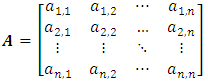 The transition matrix is engineered such that each row displays the probability of a bike moving from station i to station j, and all probabilities sum to one [9]. Mathematically, this is as follows:
 | (2) |
The state of the process, M, is set to zero, which indicates a transient state.Step 2: Transition of BikesMonto-Carlo simulation is used to select which station (j) receives a bike from the station that loses a bike (i). In the context of this research effort, there are three possible transition outcomes.Step 2A: Bike Remains in its Original StationThe first scenario is when a bike will not move from station i to station j, because the Monte-Carlo simulation selects station i to be the recipient of the bike. This situation is mathematically the following: | (3) |
This possible scenario should make sense because as the simulation moves along, some stations will retain their bikes as time passes. In fact, the transition matrix values were randomly generated such that higher selection probabilities were assigned for the ai,i values. It should be noted, however, that for bike-sharing systems of a specific nature, great care should be taken to generate reliable transition matrices. That is, it is critical that the transition matrix reflect actual system dynamics [10].Step 2B: Failed TransitionThe second scenario is when station i has no bikes (if bi = 0) to supply station j, or if station j cannot accommodate another bike (bj = C). Either of these conditions constitute a “failed” transition. If this happens, no transition takes place, and the failed transitions counter is incremented as follows: | (4) |
Step 2C: Successful TransitionThe last possible scenario is when station i and j are unique (i ≠ j), station i is not empty (bi > 0), and station j is able accommodate another bike (bj < C). When this occurs, the following updates occur: | (5) |
 | (6) |
 | (7) |
For each time increment (T), Monte Carlo selection and transition occurs for all n stations in the system. Figure 1 shows transition for one specific value of time, T.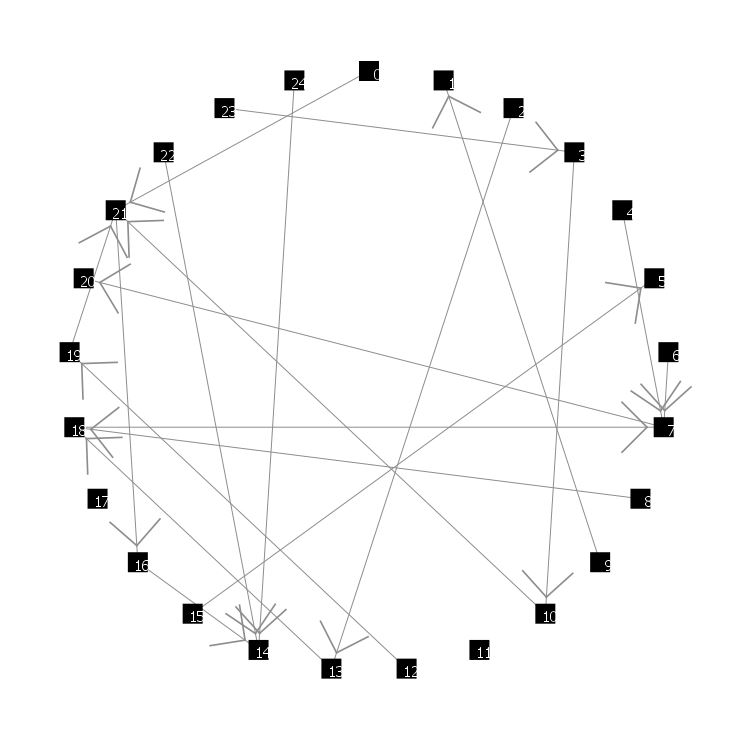 | Figure 1. Transition for a Single Time-Step |
In this figure, we see several bikes transitioning from one station to another. For example, Station 0 loses a bike to Station 21, while Station 7 loses a bike to Station 20, while gaining bikes from Stations 4, 6, and 18. Stations 11 and 17 neither gain nor lose bikes.It is important to emphasize that when bikes move from one station to another, the transition times for bikes are considered negligible.Step 3: UpdatesAfter the above-described transitions are completed, utilization statistics are calculated – specifically, system utilization and minimum utilization. System utilization, the average utilization across all stations is as follows: | (8) |
The minimum utilization is the utilization of the station with the fewest bikes. Mathematically, this is as follows: | (9) |
Utilization values for each station update as follows: | (10) |
Step 4: Re-DistributionThis step is executed if and only if the system is in a transient state (that is, if M = 0). If not (that is, if M = 1), we continue to Step 5.At this point, a check occurs to see if any stations are empty. That is, if bi = 0, station i is added to a list of empty stations. From this list of empty stations, a station s is eliminated via random selection. One station is eliminated in the presence of any empty stations. When station s is eliminated, the following occurs: | (11) |
 | (12) |
 | (13) |
 | (14) |
 | (15) |
Step 5: Steady State CheckIf the average system utilization exceeds its threshold (Uμ > Vμ) and the minimum station utilization exceeds its threshold (Umin > Vmin), the simulation is considered to be in steady state, and we proceed accordingly. We first change the state variable, M: | (16) |
We also set the steady-state time (TS) stopping time, along with the finishing time (TF) such that the steady-state simulation run length is equal to the transient-state simulation run length: | (17) |
 | (18) |
We also reset the success count and failure count at steady state as follows: | (19) |
 | (20) |
Additionally, Uμ and Umin values are recorded from the transient state.Again, the above steps are executed only if the system is found to be in steady-state. Regardless of the value of the state variable M, the time value is incremented by one: | (21) |
After incrementing the time value, we return to the transition phase, Step 2.Step 6: TerminationWhen the time increment variable, T reaches TF the simulation terminates, and we record the transition success rate, which is as follows: | (22) |
There is no need to record the utilization-related statistics, as they have not changed during the transient state, because the number of stations has not changed during the steady-state portion of the simulation.To generalize the entire simulation process, the following pseudo-code is provided: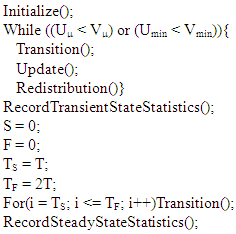
3. Experimentation
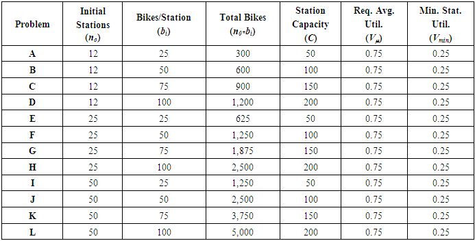
Experimentation is pursued to study the effectiveness of the simulation described above. First, it should be noted that the simulation was performed via NetLogo v. 6.0.4, an agent-based simulation package written in the Java programming language [11]. In the context of an agent-based simulation, the stations or “docks” are treated as the agents. These station-agents expand and contract in terms of the number of bikes they accommodate, and some of these station-agents disappear when it becomes apparent that their use is not as important as other station-agents. The number of bikes in the system is initialized at the beginning of the simulation, and the total number of bikes in the system never changes. The number of stations in the system does change (in the transient phase), as a function of the bikes moving from one station to another.Twelve test problems are studied to evaluate the simulation methodology. Specifically, the number of initial stations (n0), the number of bikes in each station (bi), the capacity of each station (C), stopping-threshold values 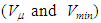 were chosen for each test problem. These user-specified values for each test problem are presented in Table 1.
Table 1. User-Specified Inputs for Test Problems
 |
| |
|
It should be noted from the table above that for all problems, the minimum threshold for average system utilization is set to 0.75, and the minimum threshold for the station with the lowest utilization if 0.25. What this means is that the transient phase of the simulation will end ONLY if the average system utilization must be at least 75%, and the station with the lowest utilization must be at least 25%. Otherwise, the transient phase of the simulation continues. It should also be noted that the utilization for all stations, and subsequently the entire system is initialized at 50% -- this is established by Equation (1).
4. Results
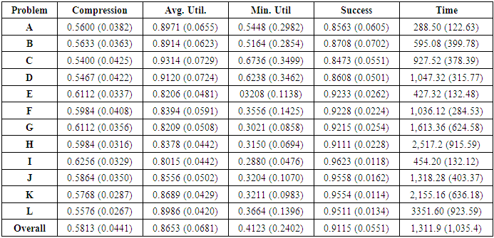
For each of the (12) test problems, the simulation was performed (25) times. This results in a data set of (300) total observations. Table 2 shows the average (and standard deviation) values of the output values for each of the (12) test problems. The bottom row of Table 2 shows the overall average (and standard deviation) of each output measure.Table 2. Experimental Results – Means (and Standard Deviations)
 |
| |
|
The average overall system utilization was 86.53%, with a standard deviation of 6.81%. The average minimum station utilization was 41.23%, with a standard deviation of 24.02%. The summary statistics from the other three outputs are reported accordingly. The overall success rate during the transient phase of the simulation is 91.15%, with a standard deviation of 5.51%. The overall success rate during the steady-state simulation phase is 59.74%, with a standard deviation of 4.79%. The success rate decreases during the steady-state phase of the simulation because there are fewer stations to accommodate the movement of bikes. If a higher success rate is desired during the steady-state simulation phase, the utilization thresholds should be lowered and/or the initial system capacity should be increased. This issue is clearly an opportunity for subsequent investigation.The size of the problem at hand deserves consideration as well. Here, the “size” of the problem is quantified by the number of bikes in the system, and it is important to consider any potential relationships between the number of bikes in the system and important simulation outputs. Figure 2 illustrates the relationship between the number of bikes in the system and utilization – both overall system utilization and station minimum utilization.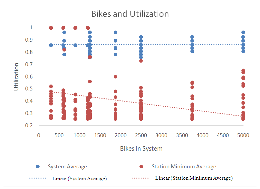 | Figure 2. Relationship between Bikes in System and Utilization |
Here we see no relationship between overall system utilization and number of bikes in the system (a flat slope), but we do see an inverse relationship between the number of bikes in the system and minimum station utilization – more bikes in the system result in the minimum station utilization being close to the minimum utilization threshold (Vmin).Figure 3 shows us that there is a positive relationship between the number of bikes in the system and the time required to complete the transient-state of the simulation.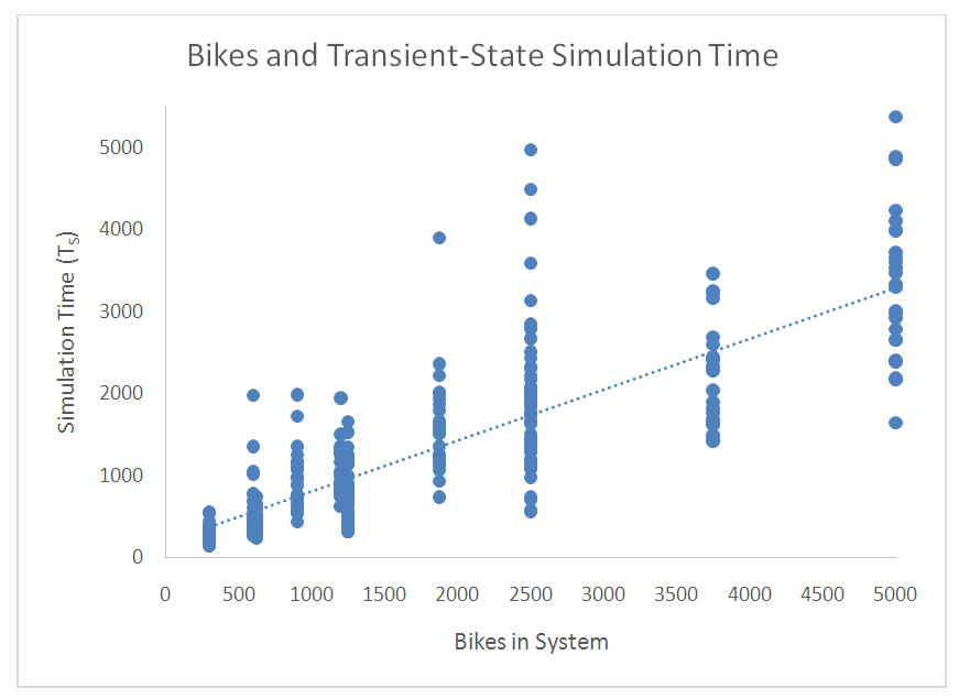 | Figure 3. Relationship between Bikes in System and Transient-State Simulation Time |
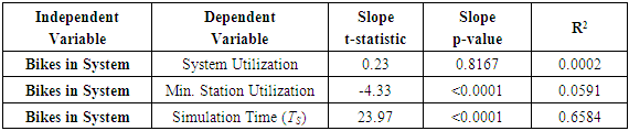
The regression statistics associated with Figures 2 and 3 are detailed in Table 3.Table 3. Regression Results
 |
| |
|
Here, we see that there is no relationship between problem size (bikes in system) and average system utilization, but there is a meaningful relationship between the minimum station utilization and the number of the bikes in the system – a negative relationship. We also see that the relationship between the number of bikes in the system and the transient-state simulation time is meaningful – a positive relationship.
5. Concluding Comments
This effort was concerned with exploiting the Markovian behavior of bikes transition from station to station in an urban environment. The intent was to design a bike-sharing system that fairly balances the tradeoff between supply of bike space and demand for bike space. The general strategy was to start with a system having excess supply, and scaling back supply as the transient-state simulation time continues. The overall system utilization is considered reasonable – a good balance of the system’s ability to supply the demand for service.Of course, with any research effort, there are opportunities for subsequent work, and this effort is no exception. Trying to design a system with a strategy other than one that starts with excess supply is an opportunity – perhaps considering user-satisfaction as an objective function value is an opportunity for study [12]. Trying stopping thresholds other than the ones used here is another opportunity for subsequent research. Adjusting the transition matrix to account for structural changes is something that also should receive consideration [13]. Non-negligible transition times for bikes transitioning from one station to another is also another research opportunity.
References
| [1] | Larsen, J. (2013) Bike Sharing Programs Hit the Streets in Over 500 Cities Worldwide, Earth Policy Institute. http://www.earth-policy.org/plan_b_updates/2013/update112. |
| [2] | Shaheen, S.A., Guzman, S. and Zhang, H. (2010) Bike Sharing in Europe, the Americas, and Asia: Past, Present, and Future. Transportation Research Record Journal of the Transportation Research Board, 2143, 159-167. https://doi.org/10.3141/2143-20. |
| [3] | Fishman, E., Washington, S. and Haworth, N. (2014) Bike Share: A Synthesis of the Literature. Urban Transport of China, 33, 148-165. |
| [4] | Larabee, M. (2009) Portland to Experiment with Rental Bike System. The Oregonian. |
| [5] | Zhang, L.H., et al. (2015) Sustainable Bike-Sharing Systems: Characteristics and Commonalities across Cases in Urban China. Journal of Cleaner Production, 97, 124-133. https://doi.org/10.1016/j.jclepro.2014.04.006. |
| [6] | Almanna, M., Elhenawy, M. and Rakha, H. (2019) Identifying Optimum Bike Station Initial Conditions using Markov Chains Modeling. Transport Findings. https://doi.org/10.32866.6801. |
| [7] | Zhao, Y., Wang, L., Zhong, R. and Tan, Y. (2018). Mathematical Problems in Engineering, Article ID 8028714, https://doi.org/10.1155/2018/8028714. |
| [8] | Chiariotti, F., Pielle, C., Zanella, A., and Zorzi, M. (2018) A Dynamic Approach to Rebalancing Bike-Sharing Systems. Sensors. Vol. 18. https://dio.10.3390/s19020512. |
| [9] | Winston, W. (2004) Operations Research: Algorithms and Applications, 4th edition. Cengage Publishing. |
| [10] | Shahsavaripour, S. (2015) A New Approach for Developing Bike Sharing, Network System. Journal of Civil Engineering Research, 5, 28-32. https://doi:10.5923/j.jce.20150502.02. |
| [11] | Wilensky, U. and Rand, W. (2015) An Introduction to Agent-Based Modeling. MIT Press. |
| [12] | Chi, Y.H. (2018) Self-Organized Bike Redistribution in Urban City. American Journal of Operations Research, 8, 386-394. https://doi.org/10.4236/ajor.2018.85022. |
| [13] | De Chardon, C.M., Caruso, G. and Thomas, I. (2016) Bike-Share Rebalancing Strategies, Patterns, and Purpose. Journal of Transport Geography, 55, 22-39. https://doi.org/10.1016/j.jtrangeo.2016.07.003. |

 Abstract
 Reference
 Full-Text PDF
 Full-text HTML