M. L. Aliyu1, U. Usman2, Z. Babayaro2, M. K. Aminu1
1Department of Mathematics and Statistics, Umaru Ali Shinkafi Polytechnic, Sokoto, Nigeria
2Department of Mathematics, Usmanu Danfodiyo University, Sokoto, Nigeria
Correspondence to: U. Usman, Department of Mathematics, Usmanu Danfodiyo University, Sokoto, Nigeria.
| Email: |  |
Copyright © 2019 The Author(s). Published by Scientific & Academic Publishing.
This work is licensed under the Creative Commons Attribution International License (CC BY).
http://creativecommons.org/licenses/by/4.0/

Abstract
This study employ a transportation model to find the minimum cost of transporting manufactured goods from factories to warehouses to (distributors). CCNN transportation data as well as OBU cement transportation data collected from BUA group of Company were utilized. The data was modelled as a Linear Programming model of transportation type and represented as transportation tableau which was solved with R Programming and TORA software version 1.0.0 to generate its initial basic feasible solution and optimal solution. From the results of the analysis, it is shown that all three methods of initial basic feasible solution (North-West corner method, Least Cost (minimum) method and Vogel Approximation method) gave varying answers. The North-West corner method gave transportation cost of ₦2,336,000, Least Cost (minimum) method gave transportation cost of ₦4,160,900 and Vogel Approximation method gave ₦2,331,800 as its transportation cost. The above result shows that Vogel Approximation method is the most efficient of all the methods because it has the least transportation cost. Another reason why the Vogel Approximation method is the best method is that, it has closest figure to the optimal solution realized after optimization. After optimization, all three methods (North-West corner method, Least Cost (minimum) method and Vogel Approximation method) gave the same result of ₦1,972,000. This shows that, all the three methods (North-West corner method, Least Cost (minimum) method and Vogel Approximation method) are optimal.
Keywords:
North-West corner method, Least Cost (minimum) method and Vogel Approximation method)
Cite this paper: M. L. Aliyu, U. Usman, Z. Babayaro, M. K. Aminu, A Minimization of the Cost of Transportation, American Journal of Operational Research, Vol. 9 No. 1, 2019, pp. 1-7. doi: 10.5923/j.ajor.20190901.01.
1. Introduction
The transportation problem is one of the subclasses of linear programming problem where the objective is to transport various quantities of a homogeneous product that are initially stored at various origins, to different destinations in such a way that the total transportation cost is at its minimum. Transportation models or problems are primarily concerned with the optimal (best possible) way in which a product produced at different factories or plants (called supply origins) can be transported to a number of warehouses (called demand destinations). The objective in a transportation problem is to fully satisfy the destination requirements within the operating production capacity constraints at the minimum possible cost. Whenever there is a physical movement of goods from the point of manufacture to the final consumers through a variety of channels of distribution (wholesalers, retailers, distributors etc.), there is a need to minimize the cost of transportation so as to increase the profit on sales. Transportation problems arise in all such cases. It aim at providing assistance to the top management in ascertaining how many units of a particular product should be transported from each supply origin to each demand destinations so that the total prevailing demand for the company’s product is satisfied, while at the same time the total transportation costs are minimized.The cost of shipping from source to destination is directly proportional to the number of units shipped. There is a type of linear programming problem that may be solved using a simplified version of the simplex technique called transportation method. One possibility to solve the optimal problem would be optimization method. The problem is however, formulated so that objective function and all constraints are linear and thus, the problem can be solved.
2. Review of Some Literatures
The transportation problem was formalized by the French mathematician (Monge, 1781).Charnes et al., (1954) developed the Stepping Stone Method which provides an alternative way of determining the simplex-method information.Dantzig (1963) used the simplex method in the transportation problem as the Primal simplex transportation method. An initial basic feasible solution for the transportation problem can be obtained by using the North West corner Rule, Least-cost or the Vogel’s Approximation method. Harold Kuhn (1955) developed and publishes the Hungarian method which is a combinatorial optimization algorithm that solves the assignment problem in polynomial time and which anticipated later primal the vest dual method. This method was originally invented for the best assignment of a set of persons to a set of jobs. It is a special case of transportation problem. Roy and Gelders (1980) solved a real life distribution problem of a liquid bottled product through a 3-stage logistic system; the stages of the system are plant-depot, depot-distributor and distributor-dealer. They modelled the customer allocation, depot location and transportation problem as a 0-1 integer programming model with the objective function of minimization of the fleet operating costs, the depot setup costs, and delivery costs subject to supply constraints, demand constraints, truck load capacity constraints, and driver hours constraints. Arsham et al., (1989) introduced a new algorithm for solving the transportation problem. The proposed method used only one operation, the Gauss Jordan pivoting method, which was used in simplex method. The final table can be used for the post optimality analysis of transportation problem. This algorithm is faster than simplex, more general than stepping stone and simpler than both in solving general transportation problem. Tzeng et al., (1996) solved the problem of how to distribute and transport the imported Coal to each of the power plants on time in the required amounts and at the required quality under conditions of stable and supply with least delay. They formulated a LP that Minimizes the cost of transportation subject to supply constraints, demand constraints, vessel constraints and handling constraints of the ports. The model was solved to yield optimum results, which is then used as input to a decision support system that help manage the coal allocation, voyage scheduling, and dynamic fleet assignment. Das et al., (1999) focused on the solution procedure of the multi-objective transportation problem where the cost coefficients of the objective functions, and the source and destination parameters are expressed as interval values by the decision maker. They transformed the problem into a classical multi-objective transportation problem so as to minimize as the interval objective function. They defined the order relations that represent the decision maker's preference between interval profits. They converted the constraints with interval source and destination parameters into deterministic one. Finally, they solved equivalent transformed problem by fuzzy programming technique.A.C. Caputo et al., (2006) presented a methodology for optimally planning long-haul road transport activities through proper aggregation of customer orders in separate full-truckload or less-than- Truck load shipments in order to minimize total transportation costs. They have demonstrated that evolutionary computation techniques may be effective in tactical planning of transportation activities. The model shows that substantial savings on overall transportation cost may be achieved adopting the methodology in a real life scenario. Chakraborty A. And Chakraborty M. (2010). Studied cost-time minimization in a transportation problem with fuzzy parameters: a case study. They proposed a method for the minimization of transportation cost as well as time of transportation when the demand, supply and transportation cost per unit of the quantities are fuzzy. The problem is modelled as multi objective linear programming problem with imprecise parameters. Fuzzy parametric programming has been used to handle impreciseness and the resulting multi objective problem has been solved by prioritized goal programming approach. A case study has been made using the proposed approach. Dhakry N. S. and Bangar A. (2013). Studied Minimization of Inventory and Transportation Cost Of an Industry” -A Supply Chain Optimization. The results they obtained from the transportation-inventory models show that the single DC and regional central stock strategies are more cost-efficient respectively compared to the flow-through approach. It is recommended to take the single DC and the regional central stock strategies for slow moving and demanding products respectively: Minimizing inventory & transportation cost of an industry: a supply chain optimization. Yan Q. and Zhang Q. (2015). The Optimization of Transportation Costs in Logistics Enterprises with Time-Window Constraints. They presents a model for solving a multiobjective vehicle routing problem with soft time-window constraints that specify the earliest and latest arrival times of customers. If a customer is serviced before the earliest specified arrival time, extra inventory costs are incurred. If the customer is serviced after the latest arrival time, penalty costs must be paid. Both the total transportation cost and the required fleet size are minimized in this model, which also accounts for the given capacity limitations of each vehicle. The total transportation cost consists of direct transportation costs, extra inventory costs, and penalty costs. This multi objective optimization is solved by using a modified genetic algorithm approach. The output of the algorithm is a set of optimal solutions that represent the trade-off between total transportation cost and the fleet size required to service customers. The influential impact of these two factors is analyzed through the use of a case study. Edokpia, R.O. and Amiolemhen, P.E. (2016). Studied Transportation cost minimization of a manufacturing firm using genetic algorithm approach. The data they obtained were analyzed and formulated into a transportation matrix with three routes and ten depots which were coded into strings after which the GA was applied to generate optimal schedules for six to nine depots that optimize the total transportation cost, revealing marked savings when compared with the company’s current evaluation method. The cost savings reduced as the number of depots in the generated schedules increased with the six-depot schedule having the highest cost saving of N347, 552 daily.The aim of this study is to minimize the cost of shipping cement from BUA cement factories to the various warehouses (Dealers).
3. Methodology
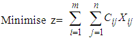 | (1) |
 | (2) |
(Demand constraint)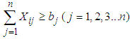 | (3) |
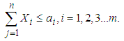
(Supply constraint)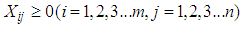 | (4) |
This is a linear program with m, n decision variables, m+n functional constraints, and m, n non-negative constraints.m=Number of sources, n= Number of destinations, ai= Capacity of ith source (in tons, pounds, litres, etc.), bj =Demand of jth destination (in tons, pounds, litres, etc.)cij = cost coefficients of material shipping (unit shipping cost) between ith sourceand jth destination (in $ or as a distance in kilometres, miles, etc.), xij= amount of material shipped between ith source and jth destination (in tons, pounds, litres etc.)A necessary and sufficient condition for the existence of a feasible solution to the transportation problem is that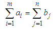 | (5) |
Remark. The set of constraints 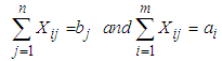 | (6) |
represents m+n equations in non-negative variables. Each variable appears in exactly two constraints, one is associated with the origin and the other is associated with the destination. Unbalanced Transportation Problem 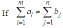 | (7) |
The transportation problem is known as an unbalanced transportation problem. There are two cases: Case (1) 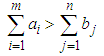 | (8) |
Case (2)  | (9) |
Introduce a dummy origin in the transportation table; the cost associated with this origin is set equal to zero. The availability at this origin is:  | (10) |
4. Data Analysis
The table 1 below, displays an individually associated cost of transporting a piece of bag from the individual supply centre (plant) to the various demand destinations, and also the demands from various destinations, as well as the supply capacity of the plants.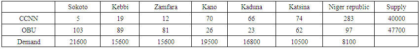 | Table 1. Transportation Tableau of the Secondary Data Collected from BUA Cement Company |
Conventionally, when we are dealing with transportation problem it is paramount to determine whether the problem in reference is balanced transportation problem or unbalanced transportation problem, which can be determined by evaluation the following scenarios (situations);1. if TOTAL DEMAND = TOTAL SUPPLY, thus the problem is balanced2. if TOTAL DEMAND ≠ TOTAL SUPPLY, thus the problem is unbalancedHowever from the Table 1, the Total Demand=107,700 and Total Supply= 87,700. Therefore in this case we are having an unbalanced transportation problem, and in the transportation problem algorithms, it is basic assumption that the problem is balanced, and hence we need to balance the problem through the introduction of dummy variable (Dummy Plant).And the supply from the dummy plant is going be given by the difference between the Total Demand and Total Supply (i.e 107700-87700=20000), thus 20000 units will assumed to be supplied by the Dummy Plant.The Table 2 below displays the balanced version of the transportation problem where the Dummy Plant takes the remaining 20000 units to be supplied, with associated cost as zero (0), and from that Total Demand is equal to the Total supply, hence the problem is balanced, and therefore we can proceed to finding the IBFS (Initial Basic Feasible Solution).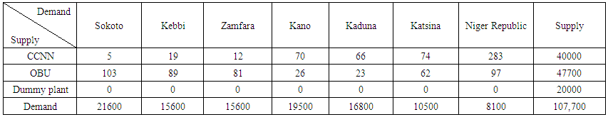 | Table 2. The Balanced Transportation Tableau |
The Table 3 below represents the result obtained as initial basic feasible solution (IBFS) by applying the North-West Corner Method. North-West Corner Method is one of the simplest methods for finding the initial basic feasible solution. In which the allocation starts from the upper left area of the table. Transportation cost is computed by evaluating the objective function which is given by:Min Z = SUM (Allocated units*Associated Cost)Min Z = 2,336,000 Therefore, total transportation cost = 2,336,000.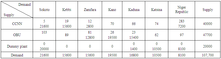 | Table 3. North-West Corner Method |
The Table 4 below represents the result obtained as initial basic feasible solution (IBFS) by applying the Least Cost Method. Least Cost Method is more reliable in comparison to the northwest corner method because it takes into account the cost of transportation during the allocation. In which the Allocation starts from the cell with the lowest transportation cost.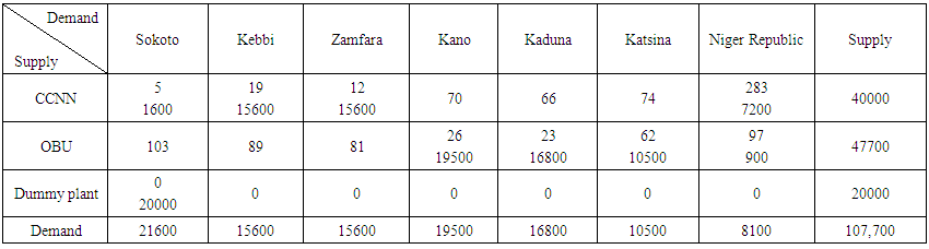 | Table 4. Least-Cost Method |
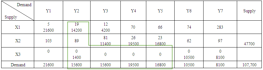
Transportation cost is also computed by evaluating the objective function:Min Z = SUM (Allocated units*Associated Cost) Min Z = 4,160,900Therefore, total transportation cost = 4,160,900.The Table 5 below represents the result obtained as initial basic feasible solution (IBFS) by applying the Vogel Approximation Method (VAM). Vogel Approximation Method is advanced version of least square method and most scholars believe VAM to be the most reliable Method in comparison with northwest corner method and Least cost method, for the fact that it does not only takes into account the cost of transportation during the allocation but rather it also considers the supply and demand before allocation could be made.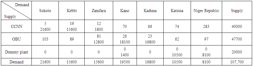 | Table 5. Vogel Approximation Method |
Transportation cost is also computed by evaluating the objective function:Min Z = SUM (Allocated units*Associated Cost) Min Z = 2,331,800Therefore, total transportation cost = 2,331,800.
4.1. Testing for Optimality
Basically, when we are solving a transportation problem the initial basic feasible solution (IBFS) cannot be considered as the optimal solution, because there may exist more better solution (which is called Basic Feasible Solution FBS) that optimize the objective function more better, and in order to evaluate whether a solution is the Basic Feasible Solution (BFS) for a particular problem, we use the optimality test to evaluate and improve the solution if there is need for improvement.The optimality test was used for all the initial basic feasible solution obtained from the various methods employed above, in order to find the optimal solution for each method. The stepping stone method was employed to test for optimality as given below:Let x’s denote plants and y’s denote the destination.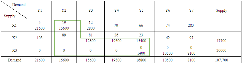 | Table 6. First Iteration |
 | Table 7. Second Iteration |
4.1.1. Optimality Test for North-west Corner Method
The stepping stone method was used, evaluating the empty cells (unallocated cells) and reallocating the cell with the highest negative. And there was a decrease on the total cost of distribution, however the optimality test still indicate that there is a need for further improvement, and thus we proceed to the second iteration.Similarly, the same sequence procedures and test were carried out after the second iteration and there were more decrease on the total cost of distribution in comparison to the first iteration, but the test of optimality still signifies that there is more better solution to be found despite the fact that there was a decrease in the total cost of distribution.Where, Min Z = 2,245,000Therefore we proceed to third iteration as given in the table 8 below.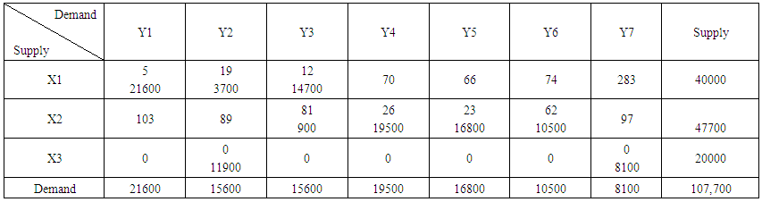 | Table 8. Third Iteration |
Table 8 shows that the optimal solution is being reached and there will be no need for further improvement again and the total cost of distribution was low in comparison to the previous iterations.Where Min Z = 1,972,000.
4.1.2. Optimality Test for Least Cost Method
We solved for Least cost method in Table 4 but here, we want to obtain the best (optimal) possible solution for the Least cost method.The optimality test after third iteration still indicates that there is a need for optimization of the solution, and hence we proceeded to the fourth iteration as given in Table 9. Table 9 shows that the optimal solution (Basic Feasible Solution) is being reached and there were a noticeable drop in the total cost of distribution in comparison to the previous iterations for the least square method.Where, Min Z= 5(21600) + 19(3700) + 12(14700) + 81(900) +26(19500) + 23(16800) + 62(10500) + 0(11900) + 0(8100)= 108000 + 70300 + 176400 + 72900 + 507000 + 386400 + 651000 + 0 + 0=1,972,000The result also shows that when using least cost method, the best allocation routine to follow would be that of Table 9 because optimum solution was reached in the fifth iteration. This allocation requires less cost compared to the other iterations.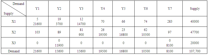 | Table 9. Fourth Iteration |
4.1.3. Optimality Test for Vogel Approximation Method
In the same way that an optimality test was carried out for the North-West corner method and least cost method we applied it on the Vogel Approximation method in order to determine the Basic Feasible Solution.Third iteration from Table 10 shows that the optimal solution is being reached and there will be no need for further improvement again and the total cost of distribution was low in comparison to the previous iterations.Where, Min Z= 5(21600) + 19(3700) + 12(14700) + 81(900) + 26(19500) + 23(16800) + 62(10500) + 0(11900) + 0(8100)= 108000 + 70300 + 176400 + 507000 + 72900 + 507000 + 386400 + 651000 + 0 + 0=1,905,300The result also shows that when using Vogel Approximation Method, the best allocation routine to follow would be that of Table 10 because optimum solution was reached in the third iteration. This allocation routine requires less cost compared to the other iterations.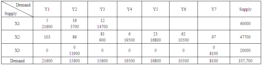 | Table 10. Third Iteration |
5. Conclusions
From the results of the analysis carried out above, it is shown that all three methods of finding initial basic feasible solution (North-West corner method, Least Cost method and Vogel Approximation method) gave varying answers. The North-West corner method gave transportation cost of ₦2,336,000, Least Cost method gave transportation cost of ₦4,160,900 and Vogel Approximation method gave ₦2,331,800 as its transportation cost. The above result shows that Vogel Approximation method is the most efficient of all the methods in finding the Initial Basic Feasible Solution because it has the least transportation cost before optimization was carried out and require less iteration compared to least cost method. And after the optimization, all the three methods (North-West corner method, Least Cost method and Vogel Approximation method) gave the same result of ₦1,972,000. This indicates that, all the three methods (North-West corner method, Least Cost method and Vogel Approximation method) can be used to find an optimal (best) solution (Basic Feasible Solution) for a given transportation problem.From the optimization tableau of Vogel approximation method, allocations of 21600 bags was made from CCNN to Sokoto, 3700 bags from CCNN to Kebbi and 14700 bags from CCNN to Zamfara. 19500 bags was allocated from OBU plant allocates to Kano, 16800 bags from OBU plant to Kaduna and 10500 bags from OBU plant to Katsina. The dummy variable allocates 11900 bags Kebbi and 8100 bags to Niger republic.This transportation model will be useful for making strategic decisions by the logistics managers at BUA Cement Company in making optimum allocation of the production from the two plants (CCNN and OBU) to the various customers (distributors) at a minimum transportation cost.
References
| [1] | Arsham, H. and Khan, A.B. (1959). A simplex type algorithm for general transportation problem: An application to stepping. Information and quantitative science, University of Baltimore, USA. Pages 219-226. |
| [2] | Caputo, A.C. (2006). The genetic approach for freight transportation planning, industrial management and data system .Vol.106, No.5. Page 719-738. |
| [3] | Chakraborty A. And Chakraborty M. (2010). Cost-time minimization in a transportation problem with fuzzy parameters: a case study. J Transpn Sys Eng & IT, 2010, 10(6), 53−63. |
| [4] | Charnes, A. and Cooper, W.W. (1954). The stepping stone method for explaining linear programming calculations in transportation problem. Management sciences 1(1), 49-69. |
| [5] | Dantzig, G.B. (1963). Programming and extension Princeton University press. Princeton. |
| [6] | Das, S.K., Goswami, A. and Alam, S.S. (1999). European journal of operational research: multi-objective transportation problem with interval cost, source and destination parameter. Department of mathematics, Indian institute of technology, Kharagpur, India. Volume 117, issue 1, pages 100-112. |
| [7] | Dhakry N. S. and Bangar A. (2013). Minimization of Inventory and Transportation Cost of an Industry”-A Supply Chain Optimization. Nonihal Singh Dhakry et al. Int. Journal of Engineering Research and Applications. Vol. 3, Issue 5, Sep-Oct 2013, pp.96-101. |
| [8] | Edokpia, R.O. and Amiolemhen, P.E. (2016). Transportation cost minimization of a manufacturing firm using genetic algorithm approach. Nigerian Journal of Technology (NIJOTECH) Vol. 35, No. 4, October 2016, pp. 866 – 873. |
| [9] | Kuhn, H.W. (1955). The Hungerian method for the assignment problem. Naval research logistics quarterly. Kuhn’s original publication 2, 83-97. |
| [10] | Shinya Kikuchi, (2000). Fuzzy sets and system. Department of civil and environmental engineering, University of Delaware, Neware, USA. Vol.116 issue 1. Page. 3-9. |
| [11] | Tony J. Van Roy, Ludo, F. and Gelder, (1980). Solving a distribution problem with side constraints. Department of industrial management, Katholieke University, Leuvan, Belgium. |
| [12] | Tzeng, G.H., Teodorovic, D. and Hwang M.J. (1996). Fuzzy bi criteria multi-index transportation problems for coal allocation planning of Taipower. European journal of operational research 95, 62-72. |
| [13] | Yan Q. and Zhang Q. (2015). The Optimization of Transportation Costs in Logistics Enterprises with Time-Window Constraints. Hindawi Publishing Corporation Discrete Dynamics in Nature and Society Volume 2015, Article ID 365367, 10 pages. |

 Abstract
 Reference
 Full-Text PDF
 Full-text HTML