1. Introduction

Queueing theory is one of the branches of applied mathematics which studies and models the waiting lines. Danish mathematician A. K. Erlang (1878–1929), who published his first paper entitled “The Theory of Probability and Conversations” in 1909 [1], is considered as the father of queueing theory. Further going back to the history, it can be observed that a viable queueing theory was developed by French Mathematician S. D. Poisson (1781–1840), who created a probability distribution function for the total outcomes of independent trials. He used statistical approach for these distributions which can be applied to the situations where excessive demands are to be fulfilled on a limited resource. During the late 1800s, all telephone calls used to be switched manually to the recipient by an operator. Each customer used to call the operator first and the operator used to fix the call for the customer. In this process, telephone companies were facing problem to appoint more operators. Callers who were unable to reach to an operator may simply hung up for several minutes with frustration and might think that it was a busy time for the operators. On the other hand, some would be waiting their turn to talk to the operator. And some others would call repeatedly thinking that the operator would be sufficiently annoyed by repeated calls to serve them next. These type of behaviour of the customers caused problems for traffic engineers because they affected the level of demand for service from an operator. A call which was not reached to the operator could be lost and could be effectively out of the system. To overcome this situation and to reduce the number of switchboards in an area, the most important application of queuing theory was developed. Those callers who repeatedly try for the operator increased demands on the system by appearing several requests. Poisson's formula was meant only for the repeated callers. Kendell [2] presented a paper that opened a general review of some points in congestion theory to enhance the study for a single server queue where input is Poisson and service time is generally distributed. In [3], he further extended the study of the stochastic processes for the theory of queues and their analysis by the method of the imbedded Markov chain. The study was carried out first reviewing on single-server queues and using the similar technique to the analysis of many server queuing system.

Stochastic process is a key factor to specify in queueing systems because it describes the arrival pattern as well as the structure and the discipline of the service facility. Queueing system deals with queue length and waiting times. The concept of queue is applied not only in the waiting system by the human beings but also in modern technology of computer and other service providers by the devices. In general, it is not necessary that service will be immediately available to address the demand of all the customers, so that they are forced to line up. In the queueing system, the one who demands the service is referred as customer, which may be a person, a task or a commodity. The other element of the queueing system is the one who provides the service with some defined discipline, called the server. It may be people, machine or objects. Some of the service disciplines are first come first served (FCFS), last come first served (LCFS), service in random order (SIRO), priority, processor sharing (PS), round-robin (RR). We study performance measures of a queueing system where only the limited number of customers are served and arrival or service or both occur in a batch. If any of the customers come after the prescribed quota has already been served, the server does not provide the service to the new comer.

The main goal of this study is to present and analyse measures of performance effectiveness for some specific queuing models. The models we investigate have important applications in the study of machine repair problem, tele-traffic, computer and flexible manufacturing systems, production processes, transportation, monitoring, controlling and managing complex engineering systems that have finite buffer system. Transient study makes the problem more realistic. The situations considered are also applicable to various day-to-day activities. It has been attracting the attention of mathematicians and operations research scientists in the field of social and liberal globalization of economy. The study provides a prospect to the development of research and design in related fields.

Rest of the paper is organized as follows: Section 2 presents the state of arts of the queueing system and associated theories developed by various researchers. Section 3 describes the different components of queueing system along with the standard notations used in queueing models. Some of the mathematical formulae for different queueing models and the derivation of simple Markovian queue are explained in Section 4. Section 5 includes Little’s law with its use for the calculation of performance measures in queueing systems. Some applications of queueing models in supply chain management are observed in Section 6. Finally, Section 7 concludes the paper.

2. Literature Review

In many practical situations, customers arrive following a Poisson stream which is an exponential inter-arrival times. Customers perform different nature coming alone or in a batch. Some are silent and wait in the queue for a long time whereas some are impatient and do not bother to leave after a while. We have noticed in our daily life also that customers wait even for a long time in the call centres until an operator is available. In spite of the different nature of customers, there are some common features on which a queue depends, namely service times, service discipline and the number of servers. These are the key factors to determine a queue. In many cases, we assume that there is an independent service time which is identically distributed with the provision of independent inter-arrival times. Among different types of queueing system, our focus is mainly on the finite capacity and batch queueing system. In finite capacity queueing system, a fixed number of customers are served and in batch queueing system, arrival and service can take place in a bulk. On top of this, we report some of the literatures in the following.

Kovalenko [4] studied rare events during busy periods along with some useful rare event theorems and singular state aggregation theorems presenting some analysis and numerical methods. Cohen and Boxma [5] gathered the information of queuing theory from its origin up to the maturity as a branch of mathematics in the field of Operations Research to calculate the performance measures. Hui [6] investigated a survey in china for five main areas namely transient behaviour, classical problems, approximation theory, model structure and applications. Fomundam and Herrmann [7] reported a survey of queuing theory application in healthcare focusing on the area of waiting time and utilization analysis, system design, and appointment systems. Lade et al. [8] used simulation of queueing system in hospitals to predict the parameters like total waiting time, average waiting time of patients, average queue length and to decrease the waiting time of patients. Shanthikumar et al. [9] carried out a survey paper on queueing theory which is applicable for semiconductor manufacturing systems. They put their efforts to improve the model assumptions and model input, mainly in averages and the variations of products. Jackson and Adelson [10] dealt with the calculation of customer characteristics in some simple cases to explain the literature for complex and practical queueing systems.

Jouini and Dallery [11] considered Markovian multi-server queue with a finite waiting line in which a customer may decide to give up for service if waiting time in queue exceeds its random deadline. They focused on the performance measures in terms of the probability of being served under both transient and stationary behaviours. Karaesmen et al. [12] examined a finite buffered queue in which the queue length is controlled by low and high service rates with higher operating cost for faster service rate. Moreover, holding cost for waiting customers to proceed and setup costs for the change in service rate were included along with some numerical examples for the validity of the model. Laxmi and Suchitra [13] studied finite buffer N-policy GI/M(n)/1 queue with Bernoulli-schedule vacation interruption, where server takes a vacation and works with a slower rate if there are less than N customers waiting for service. They used supplementary variable technique and recursive method to obtain the steady state system length distributions at pre-arrival and arbitrary epochs. Kwon [14] dealt queueing network model for the performance analysis of a flexible manufacturing system composed of workstations with limited buffers. Performance measures were developed and numerical examples were presented to verify the effectiveness of the approximation algorithm used in the model. Chakravarthy [15] illustrated numerical examples using matrix-analytic method of multi-server queueing model in which one sever is considered as the main server. The main server is connected to the other servers to provide the consultation on the FCFS basis. Ghimire and Basnet [16] studied finite capacity queueing system under the provision of vacation and service breakdown for the calculation of queue length and waiting time distributions. Yang and Wu [17] considered M/M/1/N queue with server subject to breakdowns and repairs during the time of operation where server works at a lower service rate even at the failure times. They computed transient state probabilities and some system performance measures using fourth-order Runge–Kutta method. Kaczynski et al. [18] put their effort to study M/M/s queue with initially presented k customers for the exact distribution of n^th customer’s sojourn time. Algorithms for computing the covariance between sojourn times for an M/M/1 queue with k customers present at time zero was developed using maple computer code.

Some researchers have studied and proposed some mathematical models for the nature of customers as well. Shin and Choo [29] considered an M/M/s queue in which balking and reneging customers join the virtual pool of customers called orbit. Probabilities of joining the orbit by balking and reneging customers was determined by the number of customers in the service facility. Some numerical examples were also presented to validate the results. Al-Seedy et al. [30] applied generating function technique for transient solution of system in an M/M/c queue having fixed probability for balking customers and a negative exponential distribution for reneging customers. Ayyappan et al. [31] studied single server batch service of size k considering Poisson arrival rate λ, exponential service distribution μ and Poisson catastrophe rate v to calculate the mean and variance of all the parameters described in the model. Choudhury and Medhi [32] analysed reneging behaviour where each customer is assumed to follow identical distribution of patience time ignoring the real life situations. They attempted to model a reneging property along with balking behaviour. Ghimire and Ghimire [33] dealt M/M/1 queue with heterogeneous arrival and departure with the provision of server vacations and breakdowns to evaluate some performance measures using generating function method. Atencia and Moreno [34] analysed a discrete-time Geo/G/1 retrial and without retrial queue to calculate the measure of the proximity between the system size and marginal distributions when the server is idle, busy or down. Ammar [35] obtained explicit solution of multi-server transient queue with balking and reneging behaviour of customers using similar technique of [30] along with the calculation of steady-state probabilities and some important performance measures. Gong and Li [36] developed a maximum system utility optimization model considering customer’s psychology to study the impact on their patience and rejection behaviour in a queue. They used a probability function to describe the change of customer’s psychology and rejection behaviour. Li and Cheng [37] dealt with infinite capacity queueing systems with two parallel servers having generally distributed service times where customer joined the shortest queue in the Poisson fashion. For both the queues of equal length, new arrival could join any of them with equal probability without jockeying. Shanmugasundaram and Banumathi [38] analysed multi-server queueing system using Monte-Carlo simulation to find the future behaviour of railways to reduce the queue length and system length, queue time and system time with some numerical examples.

There are some queues for which arrival and service depend on time. Those queues are known as transient queues. Singla and Garg [39] studied a feedback queueing system with correlated transient departures and calculated the transient-state queue length probabilities using Laplace Transform of the generating function. Zeng et al. [40] investigated transient M/Ek/n queuing model for the evaluation of queue length and the average waiting time of the railway container terminal gate system, as well as the optimal number of service channels during the different time period. Chan et al. [41] applied iterative and Crank–Nicolson pre-conditioner method to solve the system of linear equations for the transient solutions of M/M/2 queueing systems with two heterogeneous servers under a variant vacation policy. Jiang et al. [42] proposed free flow, slow flow and jam flow vehicle velocities in which the transitions between slow and jam flow are controlled by the duration of slow flow queues. They revealed the fact that convective instability of queueing model could generate oscillation features. Ghimire et al. [43] calculated the performance evaluations of multi-server M(t)/M(t)/n/n queuing system subject to breakdowns under transient frame work without accepting the queue of the waiting customers and verified the results using simulation. Tan et al. [44] studied transient arrival finite capacity queue where arrival rate slowly varies with time for the large capacity Probability of number of customers and mean number of customers in the system at time was calculated using asymptotic approximations approach. Kempa [45] derived explicit formulae for the queue size distribution of a finite-buffer GI/M/1/N transient queueing model. He calculated transient queue-size distribution convergence rate to the stationary distribution for the constant value given explicitly. Malligarjunan [46] evaluated performance measures and total expected cost rate for a single server queueing system under transient behaviour and entropy measures on an inventory system with two demand classes. Selinka et al. [47] developed a stationary backlog-carryover approach to compare the numerical results with simulations applicability in an analytical solution for a time-dependent performance evaluation of truck handling operations at an air cargo terminal. Ausina et al. [48] chose a single server queueing system in which Bayesian inference for the transient behaviour and duration of a busy period with general, unknown distributions for the inter-arrival and service times has been investigated.

Batch or bulk arrival and service facility is the another area of research in queueing theory. Chang and Choi [49] studied finite-buffer discrete-time Geo^X/G^Y/1/K+B queue with multiple vacations that has a wide range of applications including high-speed digital telecommunication system and various related areas presenting some performance analysis. Goswami and Laxmi [50] dealt a single server infinite or finite buffer bulk-service queues considering arbitrary inter-arrival and exponential service time distribution. The customers were served by a single server in accessible or non-accessible batches of maximum size ‘b’ with a minimum threshold value ‘a’. Ghimire et al. [51] established a bulk queueing model with the fixed batch size ‘b’ and obtained the expressions for mean waiting time in the queue, mean time spent in the system, mean number of customers/work pieces in the queue and in the system by using generating function method. Singh et al. [52] investigated retrial queue with bulk arrivals and unreliable servers providing m-optional services to observe the validity of performance measures and the effect of parameters for the queue size distribution. Banergee et al. [53] studied a single server bulk service finite capacity queue for the calculation of joint distribution of the random variables at various epochs in which service times depend on the batch size customers following Markovian arrival process. Luo et al. [54] dealt with a finite buffer Geo^X/G//1/N queue for the observation of queue-length distributions at departure, arbitrary, pre-arrival epochs with single working vacation and different input rates combining two techniques of supplementary variable and embedded Markov chain method. Claeys et al. [55] analysed a versatile batch-service queueing model with correlation in the arrival process along with some performance evaluation and buffer management.

3. Components of Queueing System

If any customer is willing to get a service, s/he should check whether a server is idle or not. If the server is vacant, customer gets the service immediately. However, if at least one customer is waiting for the service in front of each of the servers, then the new arrival should line up. Figure 1 represents the basic queueing model where the procedure of a simple queueing system is shown.

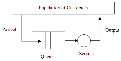Figure 1. General queueing system

From the time someone starts standing in a queue until getting served, there are certain steps to follow. These steps are called the components of a queue which are characterized by the arrival process of customers, behaviour of customers, service times, service discipline and service capacity. These components are briefly described in the followings.

3.1. The Arrival Process of Customers

The inter-arrival times are assumed to be independent having a common distribution. In many practical situations, customers arrive according to a Poisson stream (i.e. exponential inter-arrival times). Customers may arrive one by one or in batches. An example of batch arrivals is the customs office at the border where travel documents of passengers are to be checked.

3.2. The Behaviour of Customers

Customers may be patient and willing to wait for the service after some times or may be impatient and leave after a while. The behaviour of customers who leave the queue realizing that they have to wait longer than they have expected is called balking. There are some customers who leave the queue feeling that they are tired of waiting in the queue. This type of customers’ behaviour is called reneging. There is another behaviour of customers who re-join the queue which they had left earlier either by balking or by reneging, is called jockeying.

3.3. The Service Times

When a customer joins a queue, server takes a certain time to serve the customers. This time is called the service time which can be deterministic or exponentially distributed. It can also occur that service times are dependent of the queue length. For example, the processing rates of the machines in a production system can be increased once the number of jobs waiting to be processed becomes larger.

3.4. The Service Discipline

Customers can be served one by one or in batches. There are many possibilities for the order in which they enter to the service venue. Some of the service facilities are as follows:

First Come First Served (FCFS): In this process, service is provided in the order of arrival. First comer gets the service first. Generally, this method is applied in the supermarket, billing counters and many other queuing systems. It is called First In First Out (FIFO) as well.

Service In Random Order (SIRO): This is the method in which service is provided without any fixed rule. People can be observed randomly in security checkpoints. Service provider collects data randomly for statistical studies.

Last Come First Served (LCFS): It is the another method of providing service to the customers in which the last arrival gets service at first. This method is applied in the production line where the products are kept one over the other. While selling these products, the item kept at the top is sold at first though it is placed there at last.

Priorities: There can be some customers who need the service immediately for many reasons. Those customers could be in a rush or may take shorter processing time. Some emergency cases could also be there in the doctor’s clinic and some would be ready to pay more for the quicker service.

Processor Sharing: Concept of processor sharing is specially applied in the communication system where computers divide their processing power equally over all the other computers. Number of customers can get access to the internet from a single router.

Round Robin (RR): This method can be seen mainly in cyclic queueing system in which either server or the customers move in a cycle. We have experienced a revolving dining table where customers are stationary but the server moves carrying different menu on the table.

3.5. The Service Capacity

There may be a single server or group of servers to help arrivals having limitations with respect to the number of customers. For example, in a data communication network, only finitely many cells can be buffered in a switch. The determination of good buffer size is an important issue in the design of these networks.

3.6. Kendall’s Notations

To represent the behaviours discussed above, there is a standard method, called Kendall’s notation to classify different queueing systems. This is the method proposed by an English statistician D. G. Kendall (1918-2007) and is denoted by

where denotes inter-arrival time distribution, is the service time distribution, represents the number of servers and denotes the maximum number of jobs that can be occupied in the system (waiting and in service) with infinite number of waiting positions for default. Likewise, indicates queueing discipline (FCFS, LCFS, SIRO, RR etc.) having FCFS for default, and the last notation is for population size from which customers rush to the system.

For a single server queueing system, denotes the traffic intensity [56] which is defined by

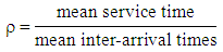Assuming an infinite population system with arrival intensity , which is reciprocal of the mean inter-arrival time, let the mean service time be denoted by , then we have

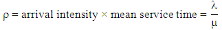If , then the system is overloaded since the requests arrive faster than they are served. It shows that more servers are needed. Let denotes the characteristic function of the event A, that is

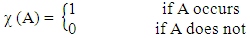Furthermore, let N(t) = 0 denotes the event that at time T the server is idle having no customers in the system. Therefore, utilization of the server during time T is defined by

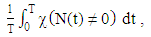where T is a long interval of time. As , we get the utilization of the server denoted by and the following relations holds with probability 1

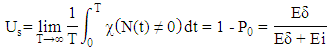where P₀ is the steady-state probability that the server is idle. and denote the mean busy period and mean idle period of the server respectively.

Theorem 1 [56]: Let X(t) be an ergodic Markov chain and A is a subset of its state space. P_i denotes the ergodic (stationary, steady-state distribution) of X(t). Then with probability 1

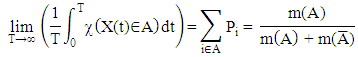where and respectively denote the mean sojourn times of the chain in A and during a cycle.

In an m-server system, the mean number of arrivals to a given server during time T is , provided that the arrivals are uniformly distributed over the servers. Thus the utilization of a given server is

The other important measure of the system is the throughput of the system which is defined as the mean number of requests serviced during a time unit. In an m-server system, the mean number of completed services is and thus

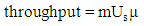However, if we consider a tagged customer, the waiting and response times are more important than the measures defined above. Let and denote waiting time and response time of the customer respectively. Clearly, the waiting time is the time a customer spends in the queue waiting for service and response time is the time a customer spends in the system, that is

where denotes service time; and are random variables and their means denoted by and , are appropriate for measuring the efficiency of the system. It is not easy in general to obtain their distribution function.

Other characteristics of the system are the queue length and the number of customers in the system. Let the random variables Q(t) and N(t) are the number of customers in the queue and in the system at time t respectively. Clearly, in an m-server system we have

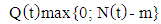The primary aim is to get their distributions which always may not be possible. In many of the situations, we have only their mean values or their generating function.

4. Formulation of Queueing Models

The important and challenging phenomena for the proposed queueing models is to express into mathematical formulation. There are different notations used to denote the queueing models. Each of the models has its specific characteristics following specific queueing discipline. For each of the queueing disciplines, there are different formulas to calculate the performance measures. Here, we describe some of the queuing disciplines with some of the formulas for their performance measures. Besides the usual notations of arrival rate and the service rate , there are some standard notations and symbols used in the queuing equations which are as follows:

C = Number of service channels

M = Random arrival/service

D = Deterministic service rate (constant rate)

With these, we describe some of the queueing models with their respective formulae in the following subsections.

4.1. Birth-Death Process

A Birth-Death process is a Markov process in which states are numbered by an integer and transitions are only permitted between two neighbouring states. Births are the cases when state variables are increased by one and deaths are the cases when state variables are decreased by one. When birth occurs, the state N moves to state N + 1 and when the death occurs, state N changes to state N - 1.

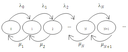Figure 2. Birth-death process

Figure 2 shows the simple birth-death process with which we can establish the balance equations as follows:

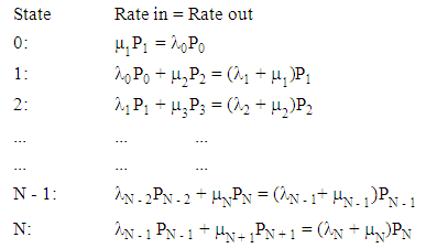All the above balanced equations can be expressed in terms of as follows:

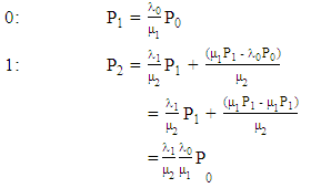Continuing this way

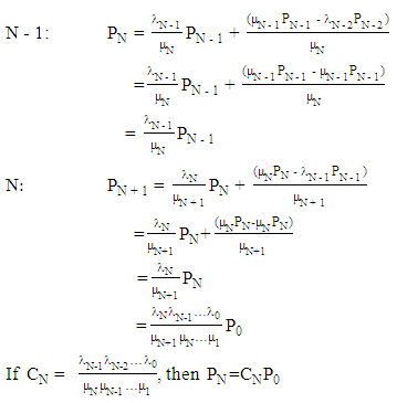
4.2. M/M/1 Queue

The queueing system M/M/1 is the simplest non-trivial queue where the customers arrive according to a Poisson process with rate , that is, the inter-arrival times are independent, exponentially distributed random variables with parameter . The service times are assumed to be independent and exponentially distributed with parameter . Furthermore, all the involved random variables are supposed to be independent of each other.

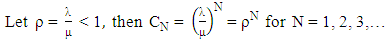Therefore, . Now, the normalizing condition is

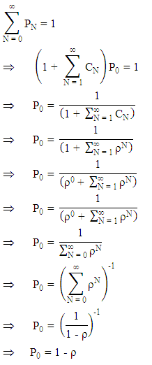Thus,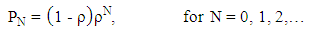

Consequently, average number of customers in the system is

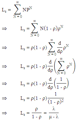Summarizing the results, we have following conclusions:

i. The probability of having zero customers in the system

ii. The probability of having N customers in the system

iii. Average number of customers in system

iv. Average number of customers in the queue

v. Average waiting time in the system

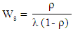vi. Average waiting time in the queue

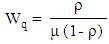
4.3. Queue

The queuing system M/M/c is the queueing discipline where c service channels are ready for the arriving customers following Poisson process. and have the usual meanings with all the random variables independent as described in the subsection 4.2. Followings are some of the formulae to for the performance measures of this model.

i. The probability of having zero customers in the system

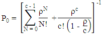ii. Probability of having N customers in the system

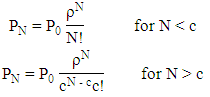iii. Average number of customers in the queue

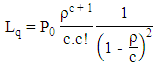iv. Average number of customers in system

v. Average waiting time in the system

vi. Average waiting time in the queue

4.4. M/M/c/k Queue

In this model, customers arrive according to a Poisson process describing independent and exponentially distributed inter-arrival times. The service times are also assumed to be independent and exponentially distributed. The difference of this model with the previous models is the only k customers who can get the service by fixed number of c servers. Followings are the formulae for some of the performance measures of this queueing system.

i. The probability of having zero customers in the system

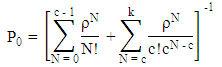ii. Probability of having N customers in the system

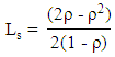
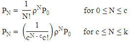iii. Average number of customers in the system

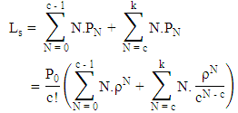iv. Average number of customers in queue

v. Average waiting time in the system

vi. Average waiting time in the queue

4.5. M/D/1 Queue

This system represents the single server queue, where arrivals are determined by a Poisson process and service times are deterministic. Some of the performance measures formulae are listed as follows:

i. Average number of customers in the system

ii. Average number of customers in queue

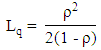iii. Average waiting time in the system

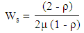iv. Average waiting time in the queue

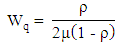
5. Performance Measures in Queueing System

Each of the proposed modes should have some kind of applications in the real life. It is important to verify those results by means of some established tools. These results are called the performance measures and are calculated by using different techniques. One of the methods to calculate these performance measures is the Little’s Law. In this Section, we briefly describe about the performance measures and the Little’s Law.

5.1. Performance Measures

Performance measures refer to the service quality as seen by the customers. There are different nature and design of the queueing models and so are the measures the performance. The main objective of proposing a queueing model is to provide the better service in minimum cost and minimum waiting time. Validity of these performances can be checked by means of simulation. There are some performance measures in the analysis of queueing models as follows:

(i) Distribution of the waiting and the sojourn times: Time spent by a customer in a queue is calculated in two categories. The first is the waiting time before starting to receive the service and the second is the sojourn time which includes the waiting time plus the service time.

(ii) Distribution of the number of customers: In a single server queueing system, there will be one customer receiving the service whereas in multiple server queueing system, there could be the customers equal to the number of servers receiving the service. Number of customers in a queueing system refers to the customers including or excluding the one or all the service.

(iii) Distribution of amount of work: It is the sum of service times of the waiting customers and the residual service time of the customers in service. Residual service time signifies the time that a new arrival waits until being served in a non-empty queue.

(iv) Distribution of busy period: When customers arrive to the server for the service, the server becomes busy. Busy period of a server is the time during which server is working continuously. While calculating the performance measures, we are interested in mean performance like the mean waiting time and the mean queue length.

5.2. Little’s Law

Little’s law states that the average number of customers in the system is equal to the average arrival rate of customer to the system multiplied by the average system time per customer [57]. This can be expressed as

where W denotes mean response time, the mean time spent in the queue and at the server, not just simply as the mean time spent waiting to be served; L refers to the average number of customers in the system and stands for mean arrival rate as usual. Little’s law can be applied when we relate L to the average number of customers waiting to receive service denoted by and W to the mean time spent waiting for service denoted by . In this sense, the other well-known form of Little’s law is

It may be applied to separate parts of much larger queueing systems, such as subsystems in a queueing network. In such a case, L should be defined with respect to the number of customers in a subsystem and W with respect to the total time in that subsystem. Little’s law may also refer to a specific class of customer in a queueing system or to subgroups of customers, and so on. Its range of applicability is very wide indeed.

Little’s law seems to be independent of [57]

• Specific assumptions regarding the arrival distribution A(t)

• Specific assumptions regarding the service time distribution B(t)

• Number of servers

• Particular queueing discipline

Little’s law is important for three reasons [57]

• It is widely applicable (it requires only very weak assumptions). It will be valuable to us in checking the consistency of measurement of data.

• It is the main task in the algorithms for evaluating several queueing network models.

• In studying computer system, we frequently find two of the quantities related by Little’s law (the average number of requests in a system and the throughput of that system) and desire to know the third (the average system residence time, in this case).

Applications of Little’s Law [57]

• On rainy days, streets and highways are more crowded.

• Fast food restaurants need a smaller dining room than regular restaurants with the same customer arrival rate.

• Large buffering together with large arrival rate cause large delays.

Theorem 2 [58]: In a closed Gordon-Newell network with m queues, write for the state of network. For a customer in transit to state i, let denotes the probability that immediately before arrival the customer sees the state of the system is Then the probability is same as the steady state probability for state for a network of the same type with one customer less.

In any of the queue, the customers want them to be served as quickly as possible. But this may not happen in all the situations. One feels quite relaxed whenever her/his turn comes for the service. To describe the nature and feeling of customers, there are some popular facts about queue. They are called Murphy’s Laws and are described as follows [57]:

• If a customer changes queue, the one s/he has left will start to move faster than the one s/he is in.

• Customer feels that her/his queue always goes the slowest.

• Whatever queue a customer joins, no matter how short it looks, will always take the longest for her/him to get served.

6. Applications of Queueing Systems

Queueing theory is applied in many of the daily life activities including computer networks, telecommunication systems, traffic flow systems, airport scheduling systems, banking and logistic operations and so on. Besides all these, queuing system is applied in the manufacturing industries as well. Items produced by industries have to be delivered to the retailers and then to the customers. If there is the proper chain to deliver those items, it can save time and money. Products of the industries can be delivered together in numbers but one machine can produce only one item at a time following a sequential order. Those produced items should be supplied to the wholesalers and to the retailers turn by turn maintaining a proper queue. In this sense, we can observe a close relationship between queuing system and supply chain management, which is described in rest of this Section.

Bhaskar and Lallement [59, 60] used the concept of supply chain to find the minimum response time for the delivery of items to the final destination through different stages of network. They identified the appropriate route of the least response time and calculated the performance measures like average queue lengths, average response times, and average waiting times of the jobs in the supply chain. They have proposed a model to calculate the mean and variance of the number of customers in the system as the follows:

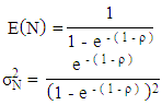where, .

Likewise, if R denotes the response time and W is the waiting time in the queue, then mean response time and the mean waiting time has been expressed as

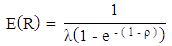and

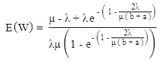Average number of jobs found on the server has been determined by the formula

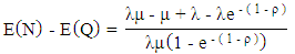Boulaksil [61] proposed a model to determine the safety stock levels in supply chain systems which are facing demand uncertainty. He reported that supply chain would meet a high level of customer service if large portion of the safety stocks are placed downstream. Teimoury et al. [62] determined holding, back ordering and ordering cost function for GI/G/1 queueing model. They proposed an inventory model for batch products along with some numerical examples of manufacturing supply chain network to analyse performance evaluation. Liu et al. [63] evaluated the performance of serial manufacturing and supply systems with inventory control by developing a multi-stage inventory queue model and a job queue decomposition approach. Then they presented an efficient procedure to minimize the overall inventory in the system maintaining the required service level. Sivakumar et al. [64] studied a discrete time inventory model to evaluate joint probability distribution of the number of customers in the pool and the inventory level where demand during stock out periods either enter a pool having finite capacity or leave the system with a predefined probability. Andriansyah et al. [65] used generalized expansion method to evaluate the performance of the systems in terms of throughput and compared results with simulation. Experiments for a large number of settings and different network topologies were also presented. They derived the formula for the throughput at node i as

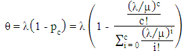where is the probability of a customer being blocked for queueing model.

Mishra and Yadav [66] considered a clocked queueing network with renewal model and used it to develop a computational approach for the analysis of cost and profit structure in the system. They found its optimality with respect to arrival and service parameters of the system. Mary and Christina [67] proposed the procedure to find the total average cost in terms of crisp values for 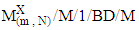with fuzzy parameters considering many other factors with some numerical example for the validity of the proposed system. Smith [68] used mean value analysis algorithm to study the material handling and transportation networks in finite buffer closed queueing system. Babadi et al. [69] applied queueing systems in nylon plastic manufacturing and recycling centres using Jackson network to minimize the average delay to deliver products, total cost and transportation cost which was checked by the sensitivity analysis by changing the parameters. Vahdani and Mohammadi [70] proposed a bi-objective optimization model in a closed loop supply chain network in which general multi-priority and multi-server queuing system for parallel processing execution has been used to minimize the cost and maximize the profit. In order to calculate the queue waiting time of arrival products into the forward flow to the bidirectional facility, following formula has been used

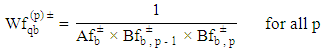where,

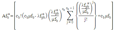for all b

and

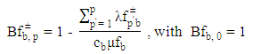The other notations used in the model are described as follows:

Waiting time in the queue of forward flow of product with priority p in bidirectional facility b;

Number of service provider at bidirectional facility b;

Service rate at bidirectional facility b for forward products;

Arrival rate of forward flow of product p to bidirectional facility b.

Diabat et al. [71] used queueing approach to determine the number and location of distribution centres, the assignment of retailers to distribution centres and the size and timing of orders for each distribution centres providing some numerical results. They proposed a model in which

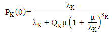Each opened distributions centres orders to the supplier when its inventory level is less than S + 1. Then the expected amount of recorders (R_K) is calculated by

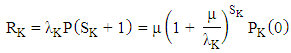On the other hand, when the level at distribution centre located at site K is equal to zero and arriving demands are lost, then the expected amount of lost sales is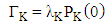

And the expected amount of inventory has been obtained by

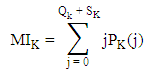where and are the recorder quantity and recorder point at distribution centre K. Wang et al. [72] collected a review defining supply chain and discussing literature in the areas, namely service supply management, service demand management and the coordination of service supply chains to observe the state in each area. He [73] derived supply risk sharing contracts for the equilibrium between the recycling price decision and the remanufacturing quantity decision using game theory illustrating some numerical examples for managerial results. Zhalechian et al. [74] studied environmental impact of sustainable closed-loop location - routing -inventory model using a stochastic-probabilistic programming approach presenting some real-world applications. Sadjadi et al. [75] derived optimization model using queuing approach for allocation of the retailers’ demands, and inventory replenishment decisions so as to minimize the total expected cost of location, transportation and inventory. Jin [76] formulated link transmission model and link queue model defining demand and supply to present queuing models for a point queue and their discrete versions.

7. Conclusions

Upon observing the contributions of the researchers in the field of queueing theory, it can be noticed that plenty of works have been done pointing out many extendable areas. Change of one parameter in any of the proposed models might cause a huge change in the result of performance measures. Small change in the arrival rate may create large queue or no queue, and small change in service rate may make the customers very happy for the quick service or may have to wait for a long time. For any of the queue, time plays a vital role. It is very important how long a customer waits in the queue to get the service and how fast a server provides the service. To make the service more effective, sometimes we need to add the servers and increase the efficiency. We have seen the proposed queueing models for finite and infinite capacities. Some of the queueing models have finite capacity and some are ready to serve for any number of customers. Some are time dependent studied under transient fashion and some are used for the optimization model. We have chosen Markovian queuing model with finite number of customers for a single or multiple servers. Besides the usual and standard mathematical modelling in queueing theory, consideration of customers’ behaviours, servers’ breakdown or vacation along with the limitation in arrivals can be introduced to make the model more realistic and challenging. On the other hand, suggesting some mathematical models considering those limitations may not always be reliable, so verifying those models in the real life situations with the use of computer simulation would be a remarkable contribution in the study of queueing theory.

All the studies carried out by the researchers have several applications in the real life. These applications are specially focused for making the life easier specially by saving time and money. In this process, number of models are proposed with applications in the different areas. The other motivation is to get the maximum profit with the minimum utilization of the limited resources, called the constraints. We intend to study the conditions for the optimal solution in order to maximize the production or the benefits using those limited constraints. These basic phenomena can be applied in telecommunication, traffic control, employee allocation, computer scheduling, supermarket, hospitals and many other fields. Variations of arrival and service disciplines in a queueing problem is the challenging work to tackle in the days to come. In addition, the simultaneous study of queueing operations with manufacturing and logistics may yield some interesting interlinks. Some of the literatures are described in the former Section. Such comparative study can be applied in the real problems of the industries to optimize production and distribution operations. The detail study of the application of queueing theory in supply chain networks will be our due course.

ACKNOWLEDGEMENTS

The first author is thankful to Erasmus Mundus SmartLink project for financial support as a PhD exchange student to carry out the work in Burgas Free University, Bulgaria from Sep 2016 – Sep 2017.

The second author is thankful to the Erasmus Mundus LEADERS Project for funding him as a Post Doc Research Fellow to carry out the work in Department of Mathematics, University of Evora, Portugal from Nov 2016 – Aug 2017.