Nalini Prava Behera, Pradip Kumar Tripathy
Department of Statistics, Utkal University, Bhubaneswar, India
Correspondence to: Nalini Prava Behera, Department of Statistics, Utkal University, Bhubaneswar, India.
| Email: |  |
Copyright © 2016 Scientific & Academic Publishing. All Rights Reserved.
This work is licensed under the Creative Commons Attribution International License (CC BY).
http://creativecommons.org/licenses/by/4.0/

Abstract
In this paper, a fuzzy inventory model for time-deteriorating items using penalty cost under the conditions of infinite production rate is formulated and solved. Penalty cost is assumed to be linear and exponential. Fuzziness is introduced in the cost component of holding cost and set up cost. Demand rate is also assumed to be fuzzy. In fuzzy environment all related parameters are assumed to be trapezoidal. Representing these three costs by trapezoidal fuzzy numbers, the optimum order quantity is calculated using signed distance method and graded mean integration method for defuzzification. Numerical examples have been given in order to show the applicability of the proposed model. Sensitivity analysis is also carried out to detect the shift in the variables of interest of the system.
Keywords:
Fuzzy Inventory Model, Trapezoidal Fuzzy Number, Defuzzification, Penalty Cost
Cite this paper: Nalini Prava Behera, Pradip Kumar Tripathy, Fuzzy EOQ Model for Time-Deteriorating Items Using Penalty Cost, American Journal of Operational Research, Vol. 6 No. 1, 2016, pp. 1-8. doi: 10.5923/j.ajor.20160601.01.
1. Introduction
Inventory control is very important for both real world applications and research purpose. In conventional inventory models, the uncertainties are treated as randomness and handled by using probability theory. The most widely used inventory model is the Economic order quantity (EOQ) model. This model was developed by Harris [1], Wilson [2]. Later Hadley [3] analyzed many inventory systems. But uncertainties due to fuzziness primarily introduced by Zadeh [4]. Zadeh et al [5] proposed some strategies for decision making in fuzzy environment. Kacpryzk et al [6] discussed some long-term inventory policy making through fuzzy-decision making models. Products like fresh vegetables, fruits, bakery items etc. do not deteriorate at the beginning of the period but they continuously deteriorate after some time. As a result, the selling price of such product decreases which can be considered as a penalty cost. Srivastava and Gupta [10] have proposed an EOQ model for time-deteriorating items using penalty cost. Fujiwara and Perera [8] have proposed an EOQ model for time continuously deteriorating items using linear and exponential penalty cost. Pevekar and Nagare [14] developed an inventory model for timely deteriorating products considering penalty cost and shortage cost. Park [7] and Vujosevic et al [9] developed the inventory model in fuzzy sense whereas ordering cost and holding cost are represented by fuzzy numbers. Margatham and Lakshmidevi [13] have proposed a fuzzy inventory model for deteriorating items with price dependent demand. Previously Park [7] has represented cost as trapezoidal fuzzy numbers, wherein Vujosevic et al [9] represented ordering cost by triangular fuzzy number and holding cost by trapezoidal fuzzy number. Jaggi et al [11] applied the extension principle to obtain the fuzzy total cost and they defuzzified the fuzzy total cost by using graded mean integration method and signed distance method. In this article, fuzzy EOQ model for time deteriorating items using penalty cost is considered where holding cost, set up cost and demand rate are assumed as trapezoidal fuzzy numbers. For defuzzification of the total cost function, signed distance method and graded mean integration method are used.
2. Definitions and Preliminaries
Definition 2.1. A trapezoidal fuzzy number  is represented with membership function
  as:
as: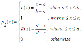 Definition 2.2. Suppose
  and
and  are two trapezoidal fuzzy number, then arithmetic operations are defined as
 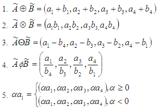 Definition 2.3. Let
 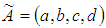 be a trapezoidal fuzzy number, then the signed distance method of
  is defined as
 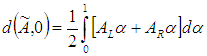 Where
Where 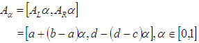 is a
is a  of fuzzy set
  which is a close interval.
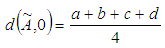 Definition 2.4. Let
 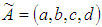 be a trapezoidal fuzzy number, then the graded mean integration representation of
  is defined as
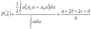
3. Assumptions and Notations
The model is developed on the following assumptions and notations.
3.1. Assumptions
(i) A single product is considered over a prescribed period of T unit of time.(ii) The replenishment occurs instantaneously at an infinite rate.(iii) No back order is permitted.(iv) Delivery leads time zero.
3.2. Notations
Q = Number of items received at the beginning of the period.D = Demand rate.H = Inventory holding cost.A = Set-up cost per cycle. µ = Time period at which deterioration of product start. C (T) = Average total variable cost per unit time.T = Length of replenishment cycle, which will not exceed product lifetime.

 by applying signed distance method.
 by applying graded mean integration method.
4. Mathematical Model (for Infinite production rate)
4.1. Crisp Model
In this context, we have considered two types of penalty cost function of age(i) Linear(ii) Exponential penalty cost functions, as a measurement of utility of the product.A linear penalty cost function 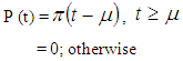 which gives the cost of keeping one unit of product in stock until age t, where µ be the time period at which deterioration of product starts and π is a constant. There will be no penalty cost incurred upon the products up to time period
  An exponential penalty cost function is taken as
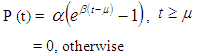 Which also gives the cost of keeping one unit of product in stock until age t, where
  be the time period at which deterioration of product starts and
  and
and  are constants.The total variable cost per cycle time consists of the inventory holding cost, set up cost and penalty cost. Since the demand rate is D unit per time.The total demand in one cycle of time-interval is T = DT.The number of items received at the beginning of the period is
  | (4.1) |
Proposed Inventory Model in Crisp SenseCase I. When linear penalty cost function is usedA linear penalty cost function 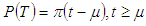 which gives the cost of keeping one unit of product in stock until age t, where
  be the time period at which deterioration of product start and
  is constant.The cost due to the deterioration of the product delivered during the period (t, t+dt) is given by
 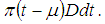 Thus penalty cost due to the deterioration of the product delivered during the time interval
  is given by
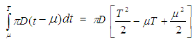 Now inventory holding cost for the period (0, T) is given by
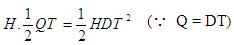 Therefore, the average total variable cost per unit time C(T) is given by
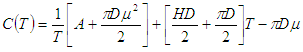 | (4.2) |
The optimal solution is obtained by differentiating  with respect to T and equating it to zero. Then the optimal cycle time
  is obtained and expressed as
 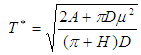 | (4.3) |
The optimal economic order quantity  is obtained by putting value of
  in eq.(4.1),
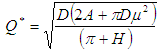 | (4.4) |
From the above expressions (4.3) and (4.4), it is clear that if there is no perishability  , then these two expression become same as that of the non-perishable lot size model.Case II. When exponential penalty cost function is usedAn exponential penalty cost function
 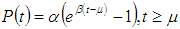 which gives the cost of keeping one unit of product in stock until age t, where
  be the time period at which deterioration of product starts and
  are constants.The cost due to the deterioration of the product delivered during the period
  is given by
 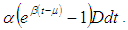 The penalty cost due to the deterioration of the product delivered during the time interval
  is given by
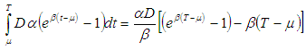 Therefore, total variable cost per unit time is given by
 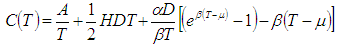 By using second order approximation of the exponential term
  in
in  We get,
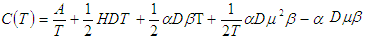 The optimal solution is obtained by differentiating
  with respect to T and equating it to zero.Then, the optimal cycle time
  is obtained and expressed as
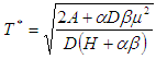 | (4.5) |
The optimal economic order quantity  is obtained by putting value of
  in eq.(4.1),
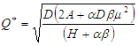 | (4.6) |
From the expression (4.5) and (4.6), it is clear that if  and
and  then these two expressions are same as (4.3) and (4.4).
4.2. Fuzzy Model
Case I. When linear penalty cost function is usedDue to uncertainty in the environment, it is not easy to define all the parameters precisely. Accordingly we assume some of these parameters  and
and  may change with some limit.Let
  and
and  are trapezoidal fuzzy numbers.The total variable cost per unit time in fuzzy sense is given by
 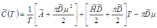 We defuzzify the fuzzy total cost
  by using signed distance method and graded mean integration method.(i) By Signed distance method, total cost is given by
 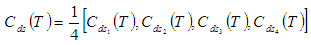 Where,
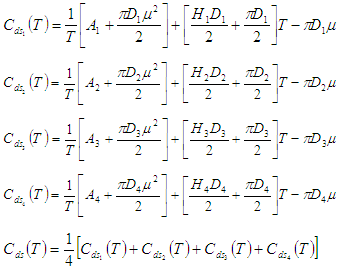 To minimize total cost function per unit time
  the optimal value of T can be obtained by solving the following equation:
 | (4.7) |
Provided  | (4.8) |
Equation (4.7) is equivalent to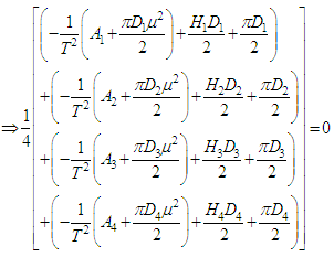 After simplification we get the optimal cycle time
  is obtained and expressed as
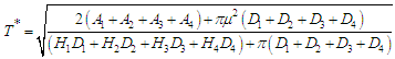 The optimal economic order quantity
  is
is  (ii) By Graded mean integration method, total cost is given by
 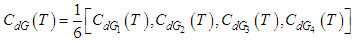 Where,
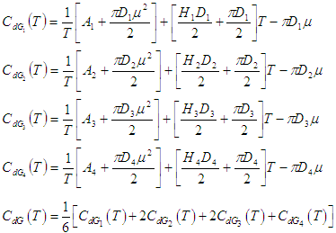 To minimize total cost function per unit time
  the optimal value of T can be obtained by solving the following equation.
 | (4.9) |
Provided  | (4.10) |
Equation (4.9) is equivalent to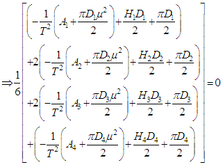 After simplification we get the optimal cycle time
  is obtained and expressed as
 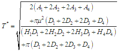 The optimal economic order quantity
  is
is 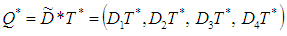 Case II. when exponential penalty cost function is used,Due to uncertainty in the environment, it is not easy to define all the parameters precisely, Accordingly we assume some of these parameters
  and
and  may change with some limit.Let
  and
and  are as trapezoidal fuzzy numbers.The total variable cost per unit time in fuzzy sense is given by
 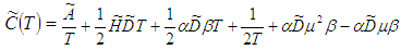 We defuzzify the fuzzy total cost
  by signed distance and graded mean representation methods.(i) By Signed distance method, total cost is given by
 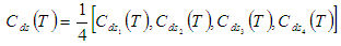 Where,
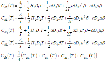 To minimize total cost function per unit time
  the optimal value of T can be obtained by solving the following equation:
 | (4.11) |
Provided | (4.12) |
Equation is equivalent to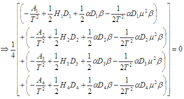 After simplification we get the optimal cycle time
  is obtained and expressed as
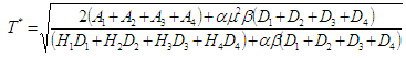 The optimal economic order quantity
  is
is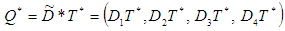 (ii) By Graded mean integration method, total cost is given by
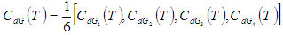 Where,
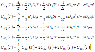 To minimize total cost function per unit time
  the optimal value of T can be obtained by solving the following equation:
 | (4.13) |
Provided  | (4.14) |
Equation (4.13) is equivalent to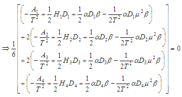 After simplification we get the optimal cycle time
  is obtained and expressed as
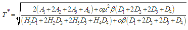 The optimal economic order quantity
  is
is 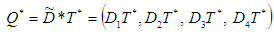
5. Numerical Illustration
The data for the study have been solicited after an intensive search of the following research papers.Tripathy, P.K. and Pradhan, S. [12]Srivastava, M. and Gupta, R. [10]Jaggi, C. K., Pareek, S., Sharma, A. and Nidhi. [11]
5.1. Crisp Model
Let P = 45 units per day, D = 30 units per day, H = Rs. 0.02 per day,  α = 10, β = 0.99, A = 100.Case-1. when linear penalty cost function is used then,Optimum cycle time
  = 5.19 daysOptimum order quantity
  = 155.7 unitsCase-2. when exponential penalty cost function is used then,Optimum cycle time
  = 4.41Optimum order quantity
  = 132.3Sensitivity Analysis of Crisp ModelThe sensitivity analysis is performed for checking the effectiveness of the EOQ model for infinite production rate with respect to the parameter µ on optimum cycle time
  and optimum order quantity
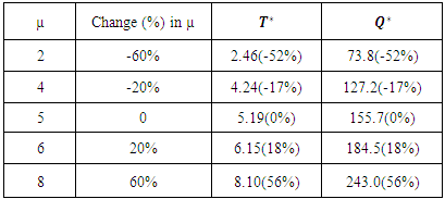
  Table 1 and Table 2 depict the values of the optimum policies for different values of the parameter µ in case of linear and exponential penalty cost. Percentage changes of these values are shown with respect to the parameter µ = 5 in the data set are taken.The Table 1 shows the effect of parameter µ on optimum policies in case of linear penalty cost. If the value of the parameter µ is increased by 60%, the value of optimum cycle time and optimum order quantity are also increased by 56%. Further, if the parameter µ is decreased by 20%, the optimum cycle time and optimum order quantity are decreased by 17%.
Table 1. Effect of parameter µ on optimal policies in case of linear penalty cost
 |
| |
|
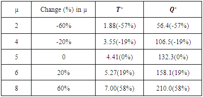
The Table 2 shows the effect of parameter µ on optimum policies in case of exponential penalty cost. If the value of the parameter µ is increased by 60%, the value of optimum cycle time and optimum order quantity are also increased by 58%. Further, if the parameter µ is decreased by 20%, the optimum cycle time and optimum order quantity are decreased by 19%.Table 2. Effect of parameter µ on optimal policies in case of exponential penalty cost
 |
| |
|
5.2. Fuzzy Model
Let P = 45 units per day, µ = 5 days, α = 10, β = 0.99,
 Case-1. When linear penalty cost function is used then, (By using signed distance method)Optimum cycle time
  = 5.18 daysOptimum order quantity
  = (103.6, 129.5, 155.4, 181.3) units(By using graded mean integration method)Optimum cycle time
  = 5.18 daysOptimum order quantity
  = (103.6, 129.5, 155.4, 181.3)Case-2. When exponential penalty cost function is used then, (By using signed distance method)Optimum cycle time
  = 5.05 daysOptimum order quantity
  = (101.00, 126.25, 151.5, 176.25) units(By using graded mean integration method)Optimum cycle time
  = 5.05 daysOptimum order quantity
  = (101.00, 126.25, 151.5, 176.25) unitsSensitivity Analysis of Fuzzy ModelThe sensitivity analysis is performed for checking the effectiveness of the EOQ model for infinite production rate with respect to the parameter µ on optimum cycle time
  and optimum order quantity
  in fuzzy sense by using signed distance method and graded mean integration method. Table-3 and Table-4 depict the values of the optimum policies for different values of the parameter µ in case of linear and exponential penalty cost. Percentage changes of these values are shown with respect to the parameter µ = 5 in the data set are taken.
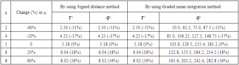 | Table 3. Effect of parameter µ on optimal policies in case of exponential penalty cost |
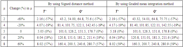 | Table 4. Effect of parameter µ on optimal policies in case of exponential penalty cost |
6. Conclusions
In this paper, a fuzzy EOQ model for time-deteriorating items using penalty cost is studied. The demand rate, holding cost and set up cost are represented by trapezoidal fuzzy numbers. It has been also fuzzified by using signed distance method and graded mean integration method.From the table-1 and table-2, it shows that if it increased the parameter  in the crisp model then the optimal cycle time and optimal order quantity will also simultaneously increase. Findings from table-3 and table-4 shows that the change in parameter
  will result in the change in
  and
and  With the increased value of parameter
  will also result in increase of optimal cycle time and optimal order quantity. Similarly, with the decreased value of parameter
  will also result in decrease of optimal cycle time and optimal order quantity. It is concluded that the value of the optimal cycle time and optimal order quantity are not much sensitive to change in the value of the parameter
  implying that fuzzy model permits flexibility in the system inputs.The outcome of this research can be extended in future to the case of discount models.
ACKNOWLEDGEMENTS
The first author is grateful to Prof. R.S. Reddy, president, ORSI, for giving opportunity to deliver this paper. Further the authors are grateful to the anonymous referees of American Journal of Operational Research for their constructive comments.
References
| [1] | Harris, F. (915) Operation and cost, Aw shaw co. Chicago. |
| [2] | Wilson, R. (1934) A scientific routine for stock control, Harvard Business Review. |
| [3] | Hardly, G. and Whitin, T.M. (1963) Analysis of inventory systems, Prentice-Hall, Englewood clipps, NJ. |
| [4] | Zadeh, L.A. (1965) Fuzzy sets, Information control, 8, 338-353. |
| [5] | Zadeh, L. A. and Bellman, R.E. (1970) Decision making in a fuzzy environment, Management sciences, 140-164. |
| [6] | Kacpryzk, J. and Stanicwski, P. (1982) Long-term inventory policy-making though fuzzy decision making models, Fuzzy sets and systems, 8, 117-132. |
| [7] | Park, K.S. (1987) Fuzzy sets theoretic interpretation of economic order quantity, IIIE Tranactions on systems, Man and Cybernetics, 17, 1082-1084. |
| [8] | Fujiwara, O. and Perera, U.L.J.S.R. (1993) EOQ model for continuously deteriorating products using linear and exponential penalty cost, European journal of operation research, 70, 104-114. |
| [9] | Vujosevic, M.et al. (1996) EOQ formula when inventory cost is fuzzy, International journal of production economics, 45, 499-504. |
| [10] | Srivastava, M. and Gupta, R. (2009) EOQ model for time-deteriorating items using penalty cost, Journal of reliability and statistical studies, vol. 2, issue. 2, 67-76. |
| [11] | Jaggi, C. K., Pareek, S., Sharma, A. and Nidhi. (2012) Fuzzy inventory model for deteriorating items with time- varying demand and shortage, American journal of operational research, 2(6), 81-92. |
| [12] | Tripathy, P.K. and Pradhan, S. (2011) An integrated partial backlogging inventory model having weibull demand and variable deterioration rate with the effect of trade credit, International journal of scientific & engineering research, vol. 2, issue. 4. |
| [13] | Maragatham, M. and Lakshmidevi, P.K. (2014) A fuzzy inventory model for deteriorating items with price dependent demand, International journal of fuzzy mathematical studies, vol. 5, No. 1, 39-47. |
| [14] | Pevekar, A. and Nagare, M.R. (2015) Inventory model for timely deteriorating products considering penalty cost and shortage cost, International journal of science technology & engineering, vol. 2, issue.2. |
| [15] | Mishra, S.S., Gupta, S., Yadav, S.K. and Rawat, S. (2015) Optimization of fuzzified economic order quantity model allowing shortage and deterioration with full backlogging, American journal of operational research, vol. 5(5), 103-110. |
| [16] | Kumar, S. and Rajput, U.S. (2015) Fuzzy inventory model deteriorating items time dependent demand and partial backlogging, Applied mathematics, vol. 6, 496-509. |

 Abstract
 Reference
 Full-Text PDF
 Full-text HTML