1. Introduction

Project management is a complex decision-making process that typically involves continuous budgeting and scheduling decisions that are made under pressures of cost and time. As the project and its environment become more complex, being subject to uncertainty, time, and money pressures, there is a greater need for efficient and smart planning and control systems to support decision-making and manage project information. Control systems need to be flexible in accepting information, instantaneous in terms of response, comprehensive in terms of the range of functions they support, and intelligent in terms of analysis and overview of information throughout the project lifecycle. Control and coordination are closely intertwined concepts in classic organization theory [22]. Recent findings highlight the principle that implementation of a control routine and coordination system influences task completion competency and thus, project management performance [19]. The main issues in designing a project planning and controlling system are:

• Determining the inspection timing throughout the lifecycle of the project (the initial planning can be considered as the first inspection). This enables monitoring the tendency to deviate from the planned trajectory while there is still time to take corrective actions.

• Assessing the remaining time and cost required for accomplishing each of the project activities, then analyzing the situation at each inspection. This enables obtaining realistic probability confidence levels of meeting project time and the cost targets.

• Optimizing the coordination when deviation from the planned trajectory is discovered. This includes re-establishing a chance-constrained time target in the most economic way, or minimizing the project completion time subject to a chance-constrained cost.

Large projects are often characterized by a combination of uncertainty and ambiguity related to goals and tasks, as well as complexity emanating from large size and numerous dependencies between different activities and the environment. Research has proved that routines work properly mostly in low uncertainty situations [12, 28], but under high uncertainty the control routine used in most production environments may not suffice [13].

Projects with ample time and generous budget, supported by appropriate control systems, can mostly be accomplished on time within budget. But, in a situation of short time float and scanty budget, attaining simultaneously both time and cost targets might be extremely difficult, because time and cost are in a trade-off relationship. In praxis, the prevalent choice is the attainment of the time target first, while the secondary objective is the satisfaction of the cost target. Thus, coordination should be mainly considered when the initial planning or present view indicates the high probability of missing the time objective, or, when the indication is that the time objective is attainable but the cost objective is not.

2. Determining the Inspection Timing throughout the Project Lifecycle

The traditional optimal control models [6, 17, 18] deal with fully automated systems where the output is continuously measured on line. The temporary nature of the project enables monitoring its advancement only at pre-set inspection points, as it is impossible to measure it continuously. Simulation studies carried out to compare the effectiveness of five inspection timing policies did not introduce significant differences (e.g., [23]). The consensus among researchers and practitioners is that there is a need for different allocations of inspections because projects can follow different patterns [3].

3. Planning and Controlling Projects by Critical Path Definition

Projects are mostly composed of partial ordered activities, while projects composed of an ordinal set of activities are very rare. The network analysis project management techniques were formed for assessing the completion of projects with partial ordered activities. Basically, the program evaluation review technique (PERT) and the critical path method (CPM) were developed along two parallel streams, one for research and development, and the other for construction, maintenance, and production. PERT considers the presence of stochastic activity durations, while CPM considers only deterministic activity durations. Actually, CPM can be considered as a special case of PERT in which all activity duration variances are equal to zero. In 1962, United States Secretary of Defense Robert MacNamara drafted an executive regulation stating that the existence of two different network-based scheduling systems was confusing, and that henceforth all Department of Defense organizations would use PERT. At the time, this appeared to enhance the development of PERT as a system, at the expense of CPM. In spite of that, by the mid 1970s the trend towards CPM was gaining momentum. Since the 1990s, differences between current versions of PERT and CPM are not necessarily as pronounced as they were originally. Current versions of PERT allow using only a single estimate of each activity duration; thus omitting the probabilistic investigation. A version called PERT/Cost also considers time-cost trade-offs in a manner similar to CPM. Currently, PERT/CPM is implemented in praxis as the precedence diagramming method (PDM). The original PERT has been essentially abandoned, rarely seen and generally only found in academic papers.

3.1. Analyzing the Situation at Each Inspection

Let denote the vector of budgets allocated to each of the project's activities, , , where and correspond to the th activity normal execution-mode, , and crash execution-mode, , respectively. The assessment of the expected project completion time related to , by PDM, relies on single estimates, most being expected activity durations, . PDM assumes that equals the expected length of the critical path (CP), , that is , where denotes the length of the path . But where uncertainty is involved, as originally considered by PERT, network paths with expected length may be longer than , and by that determine . Wherefore, the assessment of should take into consideration that there is a probability of additional project paths to determine , thereby enabling participation in the determination of . Ignoring the distributions of the activity durations and dealing with their expected durations as deterministic values is naïve. Such ignorance causes erroneous consideration that , while it is obvious that

(1)

There is a widely accepted statement that project completion time variance, , is identical to the CP variance, (see [9; 10; 21]). But it is obvious that this statement is groundless because is not necessarily identical to .

Despite the fact that uncertainty is the crux in achieving the project time target, practitioners mostly implement PDM for assessing and . Present views throughout the project lifecycle that rely on definition of CPs cause errors of being certain that the time target is attainable. In point of fact, this is actually incorrect. PDM is thereby inadequate for assessing because it may hinder exposing deviations from the planned trajectory while there is still time to take corrective actions.

3.2. Optimizing the Coordination

PERT/Cost and CPM time-cost trade-offs procedures are predominantly carried out for coordinating when the initial planning or any present view throughout the project lifecycle indicates an unperformable time or cost target. As previously noted, these procedures are based on definitions of CPs that provide an overly optimistic assessment of . Consequently, it is naïve to consider that shortening by one unit of time assures that will be shortened by one entire unit. Thus, inappropriate assurances that the project can be delivered on time, when this is not the case often leads to premature halt of the PERT/Cost procedure. The attainment of the time target (desired lead-time), , may also be impeded earlier by a premature halt that derives from the procedure's dependency on the CP concept. Because the PERT/Cost procedure considers that is determined by , when all the durations of activities lying on one of the CPs have been shortened up to investing additional budget for crashing durations of more activities seems to be disadvantageous; whereupon, at this point the crashing procedure is halted. But, crashing durations of more activities that are not lying on the alleged CP may reduce , as demonstrated by Table 1.

Table 1. The premature halt of the PERT/Cost procedure in crashing project completion

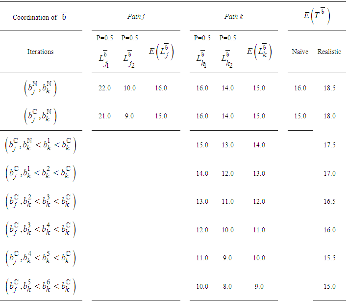
Table 1 describes an implementation of PERT/Cost procedure on a project where is 14. The project is composed of two paths, each with two probable lengths. The expected normal and crash lengths of Path j are 16 and 15 respectively, and of Path k, 15 and 7. Following PERT/Cost, at the initial state where Path j is identified as CP, which determines as 16, while the realistic calculation shows that it is 18.5. Because Path j is recognized as CP, was chosen to be shortened first by one unit of time. PERT/Cost assumes that was crashed by one unit of time, but in fact it was crashed only by a half unit. The naïve assumption of the PERT/Cost procedure is that at this stage is 15, is satisfied, and thus, the coordination is accomplished. However, the realistic is 18 and the crashing process should be continued. At this stage, disables additional shortening of related to Path j, which is considered as decisive CP, and this is what causes a premature halt of the PERT/Cost procedure. But, as we can see from Table 1, by continuing the shortening of related to Path k, which is not defined as CP, the realistic can be crashed further.

It is clear that the naïve assessment of and the premature halt of the PERT/Cost procedure disables full utilization of the coordination potential. Furthermore, as explained henceforth (Section 4.1.), the PERT/Cost procedure that omits uncertainty does not take into consideration that distributions of the activity durations may be affected by the crashing process, and by that, change the expected durations. This phenomenon may undermine the logic of the PERT/Cost procedure. These handicaps are troublesome, especially in complex networks where there are many parallel paths. Therefore, the deterministic techniques PERT/Cost and CPM time-cost trade-offs procedures seem to be inadequate when used as the basis of coordination routines.

4. Proposed Control Routine for Planning and Controlling Projects under Uncertainty

PERT relies on multiple duration estimates whose production may be time-consuming. It also requires mathematical calculations that are extremely complex. PERT provides a greater level of information to be analyzed and by that enables to quantify the risk of missing . Many analytical approximations of the distribution of project completion time, , have been developed (e.g., [4, 5, 7, 20, 24, 25, 29]), but presumably it is infeasible to compute exact results via analytic algorithms. When analytical algorithms are infeasible, Monte Carlo simulations (MC) tend to be used. MC enables receiving unbiased estimates of project completion time distribution, where other methods cannot.

An upgraded version of a model for activity durations and costs under uncertainty [16] is introduced first. We next propose a simple method for reassessing duration and cost estimates for ongoing activities at inspections throughout the controlling process, and then, our proposal for a planning and controlling routine via MC is presented.

4.1. Activity Durations and Costs under Uncertainty

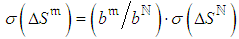
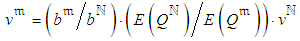
The fundamentals for stochastic time-cost trade-off models were introduced by Laslo [14]. He defined two types of duration uncertainty, the internal time uncertainty (ITU) and the external time uncertainty (ETU). The first type derives from estimates of work content, changes in technical specifications, technical difficulties, and so on, and is typical for some types of tasks such as research and development. Laslo [14] showed that when the extreme dominance belongs to the ITU aspect, the coefficient of variation of the activity duration is kept. The second type, which derives from delivery failures, weather conditions, labor unrest, and so on, is typical for other types of tasks such as production and construction. Thus, when ETU is an extremely dominant factor within the accumulative uncertainty of the activity duration, the standard deviation of the activity duration is kept during the crashing of the activity duration. Furthermore, Laslo and Gurevich [21] defined two types of cost uncertainty, the duration-deviation-independent cost uncertainty (DDICU) and the duration-deviation-dependent cost uncertainty (DDDCU). DDICU derives from an inaccurate estimate of prices, materials, and wages. The standard deviation of DDICU is proportional to the budget allocated in order to provide the desired execution-mode, that is, its coefficient of variation is preserved. The existence of DDDCU is typical for self-performed activities or outsourced activities under cost-price terms, while the absence of this dependency is typical for outsourced activities under fixed-cost terms. DDDCU derives from the dependency between the actual activity cost and random activity duration (deviations of salaries paid for random effective hours caused by ITU and salaries paid for random idle periods caused by ETU). The random DDDCU has mostly been considered as a linear function of the random activity duration [1, 2, 27]. We therefore assume that the standard deviation of DDDCU is equal to the standard deviation of the total duration distribution multiplied by the execution cost-per-time unit. The initial execution cost-per-time unit is mainly related to and varies during the crashing of the duration. The execution cost-per-time unit during the shortening of the activity duration is proportional to the change in the allocated budget. It is also inversely proportional to the change in the expected duration. (In the case of outsourced activity under fixed price terms, the duration randomness has no impact on the actual cost because the execution cost-per-time unit is considered to be zero.)

Thus, a generalized activity time-cost model that is applicable for any project activity with any feasible execution mode can be formulated as follows:

• Each with the target-effective execution duration, , requires the allocation of budget 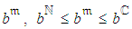, where and are known values.

• The random duration, , related to , is composed of the following random time components:

ο The random effective execution duration, , related to and affected by ITU:

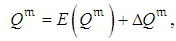(2)

where:

- The duration-budget tradeoffs, versus , are considered as pre-given continuous functions, with their estimated edge points corresponding to and respectively.

- is a random component that reflexes ITU; this variable is related to the relevant . It has zero expectation and a standard deviation proportional to ; , where is a known standard deviation of related to .

ο The random wasted time caused by disturbances, :

(3)

where:

- is considered as a known positive value.

- is a random component that reflexes ETU; the distribution of this variable does not depend on . It has zero expectation and a known standard deviation .

Thus, the random duration related to is defined as:

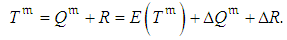(4)

• The random cost, , related to is composed of the following components:

ο , associated with .

ο A random variable that reflexes DDICU, , is related to . It has zero expectation and a standard deviation proportional to , , where is a known standard deviation of DDICU related to .

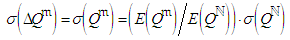
ο A random component that reflexes DDDCU equal to the deviation from the target activity duration, , multiplied by the activity execution cost-per-time unit related to , ; , where is a known execution cost-per-time unit related to .

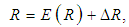
Thus, the random cost related to is defined as:

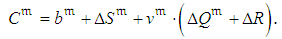(5)

Assuming some distributions for , and , the generalized model for activity duration and cost enables obtaining the simulated activity time and cost performances related to each .

4.2. Reassessed Duration and Cost Estimates for Ongoing Activities

The information obtained on the status of each ongoing activity at each inspection is limited to the initial estimated distributions of and related to known and the evidence that this activity is still unaccomplished. The cumulative distribution functions of and ( and respectively), directly follow from equations (4-5), , , , and initial estimated distributions of , , and . 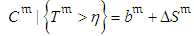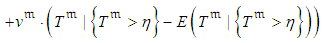Actually, at inspection the additional information concerning the ongoing activity indicates that is larger than the known value , at the moment of the inspection. Thus, at inspection the distribution of the random duration of the ongoing activity should be modified using the information that . That is, the adjusted ongoing activity duration is the conditional random variable , with the cumulative distribution function , where

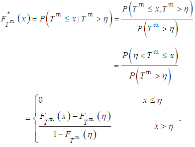(6)

Consequently, by virtue of equations (4-5), the adjusted ongoing activity cost is with the cumulative distribution function 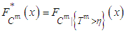, which can be straightforwardly calculated using the form of the cumulative distribution function of the adjusted ongoing activity duration, . In particular, assuming normal distributions for , , and (i.e., normal distributions for duration and cost of the project activities), the cumulative distribution function of an activity duration has the form

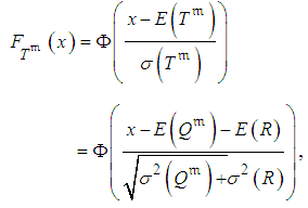(7)

where is the cumulative distribution function of the standard normal distribution. Then, the cumulative distribution function of an adjusted active activity duration (given ) is defined as

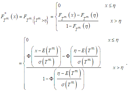(8)

Comment. Considering the problem of generating observations from the distribution defined by equation (8), we note that , where is the inverse function of the cumulative distribution function , and is a random variable uniformly distributed on the interval (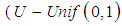). Therefore, by equation (8),

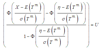(9)

or, equivalently,

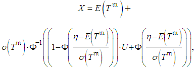(10)

where is the inverse function of the cumulative distribution function of the standard normal distribution . Thus, to generate an observation from one can generate an observation from the uniform distribution and use equation (10).

4.3. Planning and Controlling Routine via MC

The act of coordination at each inspection means regulation of execution-modes where possible by re-allocating budgets among project activities, i.e., regulating . The proposed planning and controlling routine is based on a previously developed algorithm [16], in which the activity is prioritized in receiving an additional unit of budget if it leads to maximal shortening of the simulated fractile of the project completion time, . This algorithm was found superior to an alternative algorithm where the priority for receiving additional budget was defined by the activity criticality index (ACI), i.e., the approximated by MC probability of the activity to lie on CP [8]. Assuming some distributions for , , and the generalized model (4-5) at the initial planning and at each inspection, the proposed procedure is composed of the following steps:

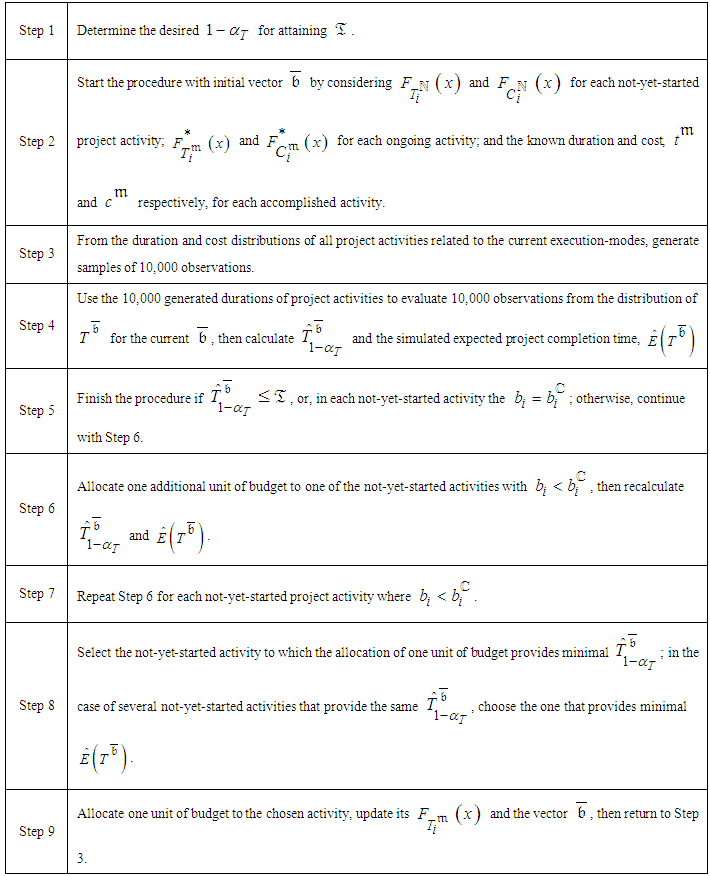Regarding the number of MC repetitions, we clarify that is obtained as a mean of 10,000 generated , is obtained as such value that 9,500 generated are less than or equal to it and 500 generated are greater than or equal to it. Note that the obtained estimator for based on 10,000 repetitions is stable (the approximate confidence interval for is and for actual projects it is reasonable to assume that . 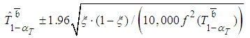The obtained estimator for is more problematic because the approximate confidence interval for is , , and 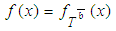is an unknown density function of (see [26]). Thus, for this estimator might not be stable enough, in which case one must consider a more essential number of repetitions. In our study we consider several , , and use 10,000 repetitions.

5. What if? Experiment

The advantage of planning projects with stochastic procedures was demonstrated by efficiency analyses on twenty-four projects [16]. Simulations showed that stochastic procedures are superior to procedures based on so-called critical paths when used to obtain lower expectation of project costs, , or any cost fractile with probability confidence level, , , subject to a pre-determined or each pre-determined . A what if? analysis on a large project (30 activities; 160 paths) with renewable resources was performed with the aim of evaluating the possible consequence of implementing alternative planning and controlling routines for delivering projects on time, and as much as possible, within budget. Assuming the generalized model (4-5) for durations and costs of the project activities as well as normal distributions for , , , project execution was simulated and accompanied by control routines based on PDM and on the proposed routine, with several pre-determined .

The simulation results for the project, as shown in Table 2, derive from a scanty budget that disables accomplishing the project on time within budget. But the proposed control routine for planning and controlling, even with modest demand for , enables the project accomplishment on time with cost overflows, while routines based on PERT/Cost cannot consume the available budget for on time project delivery. Naïve project completion assessments of PDM cause a late response to deviation from the planned trajectory, which requires drastic crashing of project completion. Drastic completion crashing, while the number of the remaining not-yet-started activities is small, mostly invokes a premature halt of the crashing procedure. Due to the fact that is quite ample, time re-establishment obstructions caused by crash execution-modes do not occur at the beginning of project execution, and as is lower, such obstructions occur later, if ever. Later, when the present view indicates attainable , the focus is turned to the cost objective, i.e., accomplishing the project on time with minimal cost. At this stage, is re-crashed in order to cut costs, but this re-crashing is obstructed by the situation of in all not-yet-started activities..

Table 2. Performances of the alternative planning and controlling routines

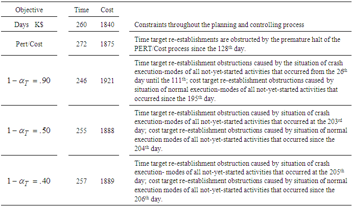
From Table 2 we can conclude post factum that the best result on time with minimal cost is provided with , but this conclusion is valid only for this specific scenario. We can also conclude that more generous budgeting will enable the accomplishment of the project on time within budget with the proposed routine, while routines based on so-called critical paths cannot accomplish the desired result on time, with any budgeting.

6. Discussion

This paper brings our attention to the fact that prevalent project planning and controlling routines based on so-called CPs are misleading in attaining the deliveries of projects on time within budget. Because computing resources are today available to everyone, project planning and controlling routines based on deterministic techniques should be replaced by more sophisticated routines. We propose such a routine for introducing realistic present views and optimizing the coordination actions that may significantly improve the chances of attaining project deliveries on time and as much as possible within budget. At any rate, project planning and controlling routines based on a stochastic approach should be always preferred, although we cannot recommend which probability confidence level may serve us best. The issue of preferable time probability confidence level seems to be unsolvable, because the choice is individual for each project, depending on the partial order of the activities, on the duration of the activities and the cost distribution, on project time and cost slacks, and especially on luck, which cannot be forecasted. However, future research may contribute additional insights and give us a more sophisticated outline for improving our choices.

Project planning and controlling routines may deal with limited capacities of project resources that require solution of a multi-mode resource-constrained scheduling (MMRCS) optimization problem. Such solution with deterministic activity durations can be very complicated [11]. Under uncertainty, the matching of activity execution with the availability of the eligible resources seems to be an impossible mission, especially where the deterministic approach provides biased timetables. Additional research in which a dynamic scheduling routine via MC (see [15]), interlocked with the proposed planning and controlling routine, will be considered; it may provide a feasible solution for this complex problem.