1. Introduction

This paper presents a method for the unconstrained minimization of the convex quadratic programming problem (QP) given by

where symmetric, positive definite matrix. This paper will be organized as follows. In section 2 we define, give the development and a detailed description of our new eigenstep method. We also prove that the eigenstep method will solve QP in at most n iterations, n being of course the number of variables of QP.

In section 3 we discuss two standard, well known optimization methods, the steepest descent method introduced by Cauchy in the nineteenth century as well as the conjugate gradient method.

Section 4 will be devoted to three more recent developments in iterative line search methods. The first being a method developed by Barzilai and Borwein[2] in 1988. Later in 2002, Raydan and Svaiter[1] extended this line of research by studying the positive effects of using over and under relaxed steplengths for the Cauchy method and introduced the relaxed steepest descent or Cauchy method. Motivated by the results of their relaxed Cauchy method, Raydan and Svaiter present a new method that is a modification of the Barzilai-Borwein method, namely the Cauchy - Barzilai-Borwein method. We also have provided references that give commentary on the above mentioned developments.

For example, in 2002 Dai and Liao[3] prove R-linear rate of convergence of the Barzilai -Borwein method and Raydan [5] establishes global convergence of the Barzilai-Borwein method in the convex quadratic case.

Finally, in section 5 we give two examples to illustrate our new eigenstep method and then we provide numerical experiments comparing all methods.

2. The Eigenstep Method

We present a method for the unconstrained minimization of the convex programming problem (QP) given by

where and Q is a n n real, symmetric positive definite (SPD) matrix. Since Q is SPD it has n real positive eigenvalues k = 0,1, …,n-1. The function f is referred to as the objective function. The vector of first derivatives of f(x) is The matrix of second derivatives of f(x) is the Hessian matrix Q. This problem is equivalent to solving the linear system and since Q is SPD and f is strictly convex our QP has a unique global minimizer

Many algorithms, for the solution of the QP use the standard iteration

where is a positive real scalar referred to as the step size and is referred to as the search direction. For convenience we use the notation to refer to the gradient of f(x) at , i.e., We say that is the optimal step size, which we will denote by

For our QP the optimal step size is given by

The following two lemmas motivate the eigenstep method.

Lemma 2.1 If is an eigenvector of Q with eigenvalue then

Proof. We know Substituting this in we obtain the desired result.

Lemma 2.2 Suppose that is an eigenvector of Q with eigenvalue 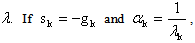then the global minimizer of f(x).

Proof. Since 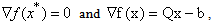we have

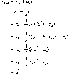Lemmas 2.1 and 2.2 suggest that for our QP if we force the step sizes at iteration k of the steepest descent method to be optimality could be attained in fewer steps.

The Eigenstep Algorithm (the eigenstep method for QP)

Calculate the distinct eigenvalues of Q denoted by k = 0,1,…, p-1,

n being the number of variables and p the number of distinct eigenvalues of Q. Arrange the eigenvalues in decreasing order,

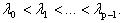Given

1. For

2. Set

3. Set

4. If the stop condition is satisfied end do,

otherwise set and go to 1.

Operated iteratively, the eigenstep algorithm initiated at point defined by the main iterative step

where each represents an eigenvalue of Q.

Remark: In order to apply the eigenstep method one must choose a step size order. In the proof of termination to follow it is evident that the order is of no consequence, thus to apply our new method we utilize an increasing step size.

Transformation to Standard Form.

Next we describe two linear substitutions that transform our objective function to standard form.

Since Q is SPD there exists an orthogonal matrix P such that

If we let x = Py we can rewrite

Letting we have transformed the objective function to

We now set to obtain

Letting and ignoring the constant

(it does not affect the value of the minimizer we have transformed the objective function to standard form

The next lemma shows a one to one correspondence between the minimizers of our QP and our QP in standard form.

Lemma 2.3 if and only if

is the unique global minimizer for f(x).

Proof. We know 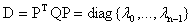is non-singular therefore

Since, 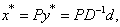we have

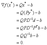Conversely, assume is the unique global minimizer for f(x), thus

and

The next theorem sets the stage for our general proof which follows.

Theorem 2.1 The eigenstep method will solve a QP in standard form in at most n iterations.

Proof. The QP to be solved is min Let be arbitrary but fixed. The eigenstep method gives the iterates

Continuing we see that

The i-th row of is a zero row since the diagonal element is

Thus, the product is the zero matrix and it follows that the global minimizer.

Proof of Termination

Theorem 2.2 The eigenstep method will solve our QP in at most n iterations.

Proof. We will show a one to one correspondence between the iterates of the eigenstep method applied to our QP and the iterates of the eigenstep method applied to our QP in standard form. The result will then follow from Theorem 1.

We proceed by induction. Let be arbitrary but fixed, and let

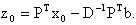Assume that for

We have

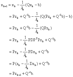A practical motivation for the introduction of Eigenstep method is that it not only solves the QP in at most n iterations, but also saves the computation in each iteration. Since the eigenvalues of Q are fixed for the problem and do not vary in each iteration, we can pre-calculate them before performing the iterative programming. The total computation complexity in iterations is the cheapest compared with all other methods presented in this paper.

3. Standard Methods

The Steepest Descent Method.

The steepest descent method uses as the search direction since is a direction of steepest descent and uses the optimal step size. For instances of the QP in which the eigenvalues of the Hessian have different orders of magnitude, it is known that the steepest descent method can exhibit poor performance. Our research has shown that this poor performance is due to the choice of steplength not the search direction. Our attempts to alter the steplength of the steepest descent method in order to improve its performance gave birth to the new eigenstep method .

The Conjugate Gradient Method.

Early attempts to modify the steepest descent method led to the development of this method which can be shown to solve our QP in n steps using again our standard iteration. This method gets its name from the fact that it generates a set of vectors that are conjugate with respect to Q that is, 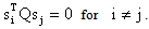In the case where Q = I the conjugate vectors are just orthogonal vectors. The method is initialized by being given, while

4. Recent Developments

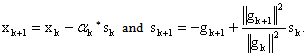
In 1988 Barzilai and Borwein[2] presented alternatives to the optimal step size. They introduced a nonmonotone steplength which avoids the drawbacks of the steepest descent method. The Barzilai-Borwein method for the unconstrained minimization problem can be written as

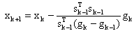
where For QP the Barzilai-Borwein method reduces to is the optimal choice of the steepest descent method at the previous iteration.

Relaxed Steepest Descent Method (RSD)

Inspired by the work of Barzilai and Borwein, Raydan and Svaiter[1] introduced two new methods which will be discussed in this paper.

The first method developed by Raydan and Svaiter in[1] is a modification of the steepest descent method applied to QP. They alter the optimal steplength using over and under relaxation parameters between 0 and 2. The authors have shown that by multiplying the optimal step size by a relaxation parameter between 0 and 2, one can improve the performance of the Cauchy or steepest descent method.

Recall that the classical steepest descent method applied to QP is

where and the optimal choice of steplength is given by

More specifically, Raydan and Svaiter modify the steepest descent method by introducing over and under relaxation parameters. Taking the relaxation parameters as a random scalar with a uniform distribution on[0 , 2], we get

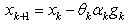Notice that for we obtain the classical steepest descent method, and also that for

Raydan and Svaiter prove in[1] that the sequence of points generated by the RSD method converge to the optimal solution and show that relaxation might be a suitable tool to accelerate the convergence of the steepest descent method . They illustrate their findings with numerical experiments.

The Cauchy-Barzilai-Borwein method (CBB)

Motivated by the Barzilai-Borwein method, Raydan and Svaiter propose a combination of the steepest descent method and the Barzilai-Borwein method for which a Q-linear rate of convergence can be established in a suitable norm. The new method is called theCauchy-Barzilai-Borwein (CBB) method[1], which can be obtained as follows:

,

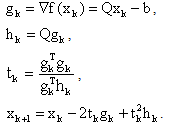They show that the CBB algorithm is much more efficient than the classical steepest descent and the RSD methods using extensive numerical experiments.

5. Examples and Numerical Experiments

Example 5.1

Consider the QP minimize

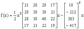Our solution is, 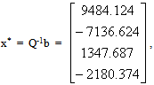f(x^*) = -1462685.7187.

The eigenvalues of Q are

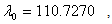
We begin our algorithm with

Iteration 0

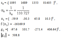Iteration 1:

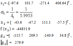Iteration 2:

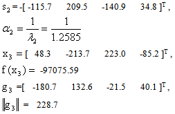Iteration 3:

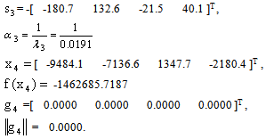Also for this example the steepest descent method terminated after 14695 iterations with a CPU time of 84.98 seconds compared to a CPU time of 0.22 seconds using the eigenstep method.

Example 5.2

In this example in which we illustrate with figure 5.1 we compare the performance of; the steepest descent method, the conjugate gradient method , the CBB method, the RSD method and the eigenstep method (E) in the solution of

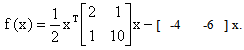Our minimizer is x^* =[ -1.78947 -0.42105 ]^T

Note that all 3 methods have the same search direction after the first iteration. The steepest descent method and the conjugate gradient method also have the same step size, ^* and arrive at the same point after the first iteration, however the eigenstep method has a shorter step after the first iteration. Next, the conjugate gradient method and the eigenstep method terminate with x^* after iteration two and the steepest descent method produces a zig zag route to x^* terminating after 31iterations to x^* with a tolerance of

The following graph illustrates the CBB RSD and eigenstep methods also applied to example 5.2.

Numerical experiments for smaller problems

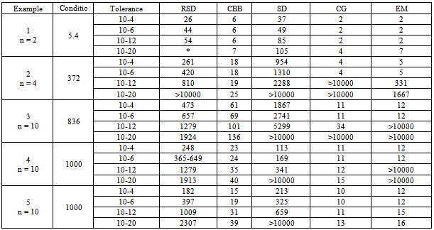
In table 5.1 we used matlab to randomly generate matrix Q and implement the RSD, CBB, steepest descent (SD), conjugate gradient (CG), and eigenstep (EM) methods for small problems For the eigenstep method, we pre-calculated the eigenvalues of the Q, we then sorted them in descending order and started our algorithm applying the main iterative step (see definition 2.1)starting with the largest eigenvalue. 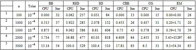The stop rule is either the number of iterations is greater than 10000 or the norm of is less than the tolerance. The condition number is the ratio of the maximum eigenvalue to the minimum eigenvalue of Q. The data under each method are the number of iterations required to obtain the optimal solution. The CPU times were too small to be relevant.

If the tolerance is not required to be very small (say 10^-4~10^-6), the number of iterations of the eigenstep and conjugate gradient methods are equal to the dimension of the problem. For most practical applications, these tolerances are adequate.

Theoretically we have proven and we know that the conjugate gradient and eigenstep methods terminate in at most n iterations. The reason that finite termination is not satisfied with a very small tolerance (say 10^-12~10^-20), is that the floating number computation and rounded arithmetic leads to subtle discrepancies (see[6, p.389]).

Numerical experiments for large problems

In table 5.2 we again used Matlab to implement the Barziai-Borwien (BB), RSD, CBB, steepest descent (SD), conjugate gradient (CG), and eigenstep (EM) methods to solve larger problems. We first used matlab to randomly generated the matrix Q, the vector b and the initial point x₀ and saved this data in a binary data file. Before running the methods, all data are read from the data file to ensure all methods are used to solve the same problem. In each iteration, to obtain good performances for these large problems, we coded a step in the algorithm that ensures that the function value is decreasing. The CPU time of Eigenstep is the sum of the time of iterations and the time of precalculating the eigenvalues. All these experiments were performed by a PC: Intel Pentium 4, CPU 3.2GHz 1.0GB of RAM.

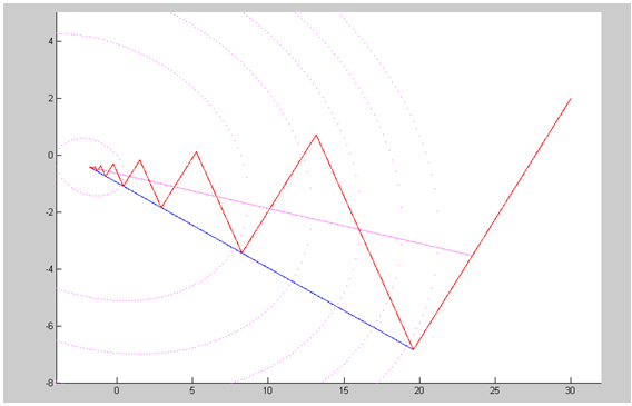Figure 5.1. Steepest descent (red),conjugate gradient (blue), eigenstep (purple) methods

Table 5.1. A comparison of five methods with n=2, n=4 and n=10

Table 5.2. A comparison of six methods with n=100, n=1000, n=2000, n=3000

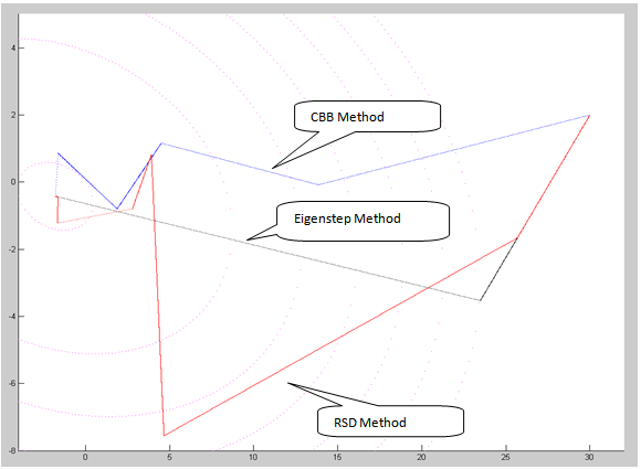Figure 5.2. RSD, CBB and eigenstep methods

6. Conclusions

In this paper we presented theorem 2.2 which validates the proposed eigenstep method to solve our model problem. We compared the eigenstep method to other well known first order methods. The conjugate gradient method and the eigenstep method both terminate in at most n iterations and our experiments show that both methods are superior in performance to the classical steepest descent method. Future work may include modifying the eigenstep method to deal with more general functions. For example, for a function where the Hessian is not constant one might consider using using the reciprocal of the largest eigenvalue as a step size to move efficiently to the next point. In fact modifications of the conjugate gradient method along with step size formulas by Fletcher-Reeves and Polak-Ribiere[6, p.399] are used today to deal with more general problems since these methods have low storage requirements.