-
Paper Information
- Next Paper
- Paper Submission
-
Journal Information
- About This Journal
- Editorial Board
- Current Issue
- Archive
- Author Guidelines
- Contact Us
American Journal of Operational Research
p-ISSN: 2324-6537 e-ISSN: 2324-6545
2013; 3(2): 28-44
doi:10.5923/j.ajor.20130302.02
An Exact Method for Solving the Four Index Transportation Problem and Industrial Application
 Abstract
 Reference
 Full-Text PDF
 Full-text HTML
Tuyet-Hoa Pham1, Philippe Dott2
1Graduate School SPI, Cézeaux Campus, Blaise Pascal University, 63173, Aubière Cedex, France
2IREM, UMR 6158, Cézeaux Campus, Blaise Pascal University, 63173, Aubière Cedex, France
Correspondence to: Tuyet-Hoa Pham, Graduate School SPI, Cézeaux Campus, Blaise Pascal University, 63173, Aubière Cedex, France.
| Email: |  |
Copyright © 2012 Scientific & Academic Publishing. All Rights Reserved.
Due to the importance of freight transport in the panel of logistics cost, our research is conducted to optimize transportation on cost criterion. Its aim is to find a solution on the minimum transportation cost for the four index transportation problem (4ITP: origin, destination, goods type, vehicle type). The 4ITP was solved by Ninh’s method where the problem is not degenerated and the solution existence condition (SEC) is verified. Given the complexity of such a model, we develop an exact method to solve this problem with real variables in all untreated cases where it is degenerated and the SEC is not satisfied. On the criterion of degeneration treatment capacity and execution time, our method takes more advantages over the simplex. Based on the obtained result, we propose an extension used the elements in FORTRAN 95 library to integer and mix variables, which matche the piece and weight transportation model. This will be a key factor to the implementation of this four index model in industry.
Keywords: Degeneration, Four Index Transportation Problem, Potential Method, Integer Variable, Real Variable, Simplex Method
Cite this paper: Tuyet-Hoa Pham, Philippe Dott, An Exact Method for Solving the Four Index Transportation Problem and Industrial Application, American Journal of Operational Research, Vol. 3 No. 2, 2013, pp. 28-44. doi: 10.5923/j.ajor.20130302.02.
Article Outline
1. Introduction
- The study of road freight transport includes all the methods and activities which aim is to coordinate the physical flows by optimizing all intervening in each link of the chain. Since the first classical problem, defined as the two index transportation problem (2ITP), was developed in 1941 by Hitchcock, the research in this area has achieved satisfactory results on various extensions. There are two main directions of research: theoretical and operational research. On the theoretical point of view, the research on transportation problem is developed at the macro level with the n index problem. On the operational angle, the results are still limited because the application of transportation models to the reality is complex. Consequently, the remaining problem is to find methods to solve the particular problems.A classification of transportation problems can be determined based on the typology of index number and corresponding resolution method. We classify them into four groups: 2 indexes, 3 indexes, 4 indexes and n indexes. In this paper, we are interested in the four index transportation problem, called 4ITP with four indexes: origin, destination, goods types and truck types, one of extension cases of the Hitchcock’s problem. The 4ITP includes the exchange of one or several goods types transported by vehicle types in a single link between origins to destinations.This article is organized as follow: in the first part, we present the economical signification and the formalization of 4ITP. Subsequently, we give a brief literature review and explain the relationship with our problem. In the third part, we propose an exact method, an extension of Ninh’s method (Ninh, 1979), to solve the 4ITP in all particular cases. To illustrate this method, we also present the obtained execution results on the artificial database. Based on it, we compare the performance of our method with the simplex. Finally, an approached method used to solve the 4ITP with integer and mix variables will be proposed. We also develop a program on the integer four index model in Fortran 95 by coupling between this algorithm and the main program of 4ITP with real variable. This will be the first test for the implementation of our algorithm with real industrial data.
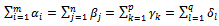
2. Problem Presentation
2.1. Economical Signification
- In the large economic zone, there is a group O with m production sites that manufacture p product types. These products are raw materials for the manufacturing network of its customer D. The group O can possess q vehicle types or use the provider transportation service to transport the goods. The maximum quantity that a vehicle type Hl can load is
 (ton, e.g.). The production network of group D uses the flow “just-in-order” to avoid the storage of raw materials in the manufacturers. Therefore, these raw materials are stored in a logistics network that consists of n warehouses. To maintain the production flow, the manufacturing sites send their requests on raw materials to the management centre. Based on this obtained database, the centre can calculate the ordered total quantity of product type Sk is
  (ton, e.g.) and then sends the order to its subcontractor, group O.Note that the production site of subcontractor is Oi (i=1...m) and these are called origins. The warehouse of customer is Dj (j=1...n) and these are called destinations. The product type Sk (k=1...p) and the vehicle type Hl (l=1...q). The quantity of goods (all types of existing products to this site) that the site Oi is ready to deliver is
  (ton, e.g.); the storage quantity of the warehouse Dj is
  (ton, e.g.); the management centre demands to be supplied enough
  tons of product Sk for its total network while
  must have the same calculation unit.
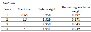
 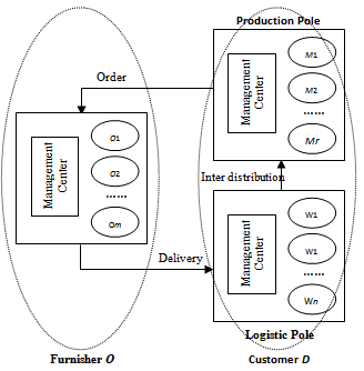 | Figure 1. Order and delivery system between Furnisher O and Customer D |
2.2. Model
- The 4ITP formalization is elaborated with the following data:→ m origin nodes
 . The goods delivery capacity of this node is
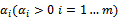 .→ p goods types. The total quantity of goods type
 at all the nodes is
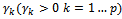 .→ n destination nodes
 . The reception capacity of goods at this node is.→ q vehicle types. The total quantity of goods that the vehicle type
  can transport is
 .→
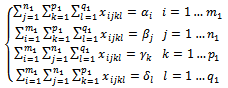
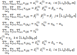
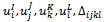
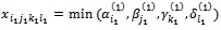
.→ the unit transportation cost for a unit of goods type Sk that is transported from origin node Oi to destination node Dj using the vehicle type Hl.The hypothesis must be fixed by inhibition for the transport of goods in the direction from destination nodes to origin nodes. The variables of 4ITP are
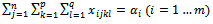
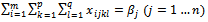
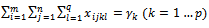
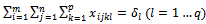
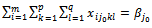
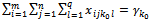
 the quantity of goods type Sk is transported from node Oi to node Dj by the vehicle type Hl in the solution to establish.The problem becomes: Determine the variables
 | (1) |
 | (2) |
 | (3) |
 | (4) |
 | (5) |
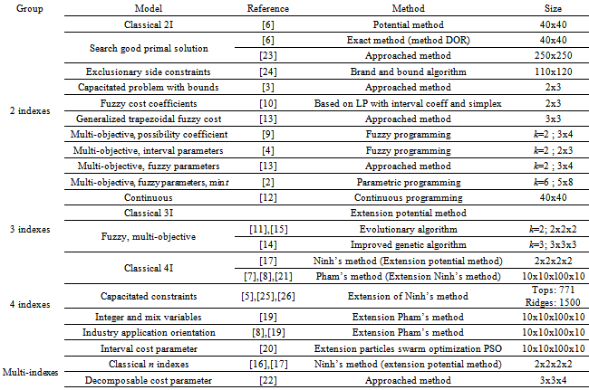
3. Literature Review
- The first transportation problem, also called the two index problem (2ITP) or the foundation to research the classical transportation problem, was developed in 1941 by Hitchcock. The first resolution method defined by Kantorovich and Gavorin, Russian researchers, is the potential method. Then, G.B. Danzig proposed another method for solving the classical problem based on the simplex method. In 1958, Gleyzal presented a method using the dual simplex algorithm, and in 1963, Kuhn proposed a method for solving the allocation problem, a special case of transportation problem, by developing the idea of a Hungarian mathematician in 1931. Although other methods have been introduced so far, the potential method is the most commonly used method in research and teaching.A classification of extension on the Hitchcock’s problem is based on the typology of index numbers and resolution methods. Four groups are arranged: 2 indexes, 3 indexes, 4 indexes and n indexes.
3.1. Two Indexes Transportation Problem Group
- In order to solve the Hitchcock’s problem, the most commonly used method is the potential method. They used a rectangle: one side represents origins. They divided this side into m segments and the ith segment represents origin Oi (i=1…m). The other side represents destinations. They also divided it into n segments and jth segment represents destination Dj (j=1…n). Each cell of the table represents an arc (ij) in which, they noted the cost cij and goods xij. Then, they calculated the potentials and tested the optimality criterion. If the solution is not optimal, this solution is improved to obtain the other better solution. The first branch focuses on the way to find a good initial solution. There are several new methods proposed, for example, an exact method DOR[6] and an approached method which obtains a very good initial solution (with a less ecart than 2% on the dual problem) for the primal problem whose execution time is O(n3)[23]. The method DOR is very special. Being different from the previous methods (determine the boxes consisting of distributed goods with the minimal transportation cost), Dubeau and Gueye determined the boxes with a high cost: determine the boxes (i,j) in which the goods are not delivered , i.e. xij=0, then determine the boxes in which a minimum goods quantity must be assigned and continue until the first solution. On the performance of this method, the researchers found that it is more effective than the Vogel Russel method and in many cases of small size, the DOR method immediately gives the optimal solution.The second branch consists in a constraint on the limited transportation capacity on the roads. The problem treated the bound on total availabilities at sources and total destination requirements. The application domain was found in a variety of real world problems such as: telecommunication networks, production-distribution system, rail and urban road system, planned automated cargo system with finite capacity of resources, for example, vehicles, docks, parking places, ...[3]. Another extension in this branch was the problem with exclusionary side constraints, a practical distribution and logistics problem: a warehouse may be unable, or may not be allowed, to receive goods simultaneously from some pairs of sources due to the damage or possible deterioration, e.g hazardous materials such as explosives, flammables, oxidizing elements should be separated from the others in order to avoid the accidents[24].In the third branch, the linear objective function is kept but the unit transportation cost is fuzzy, the offer and the demand are fuzzy and integer. Several algorithms were proposed to solve these transportation problems in a fuzzy environment but until now, no one has used generalized fuzzy numbers for solving them. So, an extension was proposed for solving a special type of fuzzy transportation problem by assuming that a decision maker is uncertain not only about the precise values of transportation cost but also the supply and demand of the product. This is a case in which transportation costs are represented by generalized trapezoidal fuzzy numbers[13]. In the fourth branch, the transportation system must respond to multiple objectives. Thus, the linear objective function is also kept but the mono-objective problem is transformed into multi-objective one. Following this extension, the problems were developed: the possibility coefficient of objective function[9], interval parameters[4] and interval-valued fuzzy parameters[13].The fuzzy programming was essentially used to solve them. The fifth branch consists of the solution on the mass transportation problem, a typical example in the continuous programming, which was proposed at the first time by Monge in 1871. It was discretized by Hitchcock to become the 2ITP. Then, Kantorovich introduced the problem under geometric form and Kangabo used the continuous programming to solve it[12].
3.2. Three Indexes Transportation Problem Group
- By increasing the index numbers, the three index transportation problem (3ITP) was developed and solved by an extension of the potential method, under the geometric form. These properties are source, destination and type of product or mode of transportation. Its extensions were less varied: a new approached method, based on adding additional parameters to create a new deterministic problem, was proposed to solve the interval problem. For the fuzzy problem, a simple approached method based on transforming this problem into interval problem and an evolutionary algorithm based parametric approach are presented[11]. In addition, an improved genetic algorithm was proposed for solving multi-objective problem in which the coefficients of objective function were represented as fuzzy numbers[15]. With the use of the parallelepiped, we see that the constraints of the three index problem can be represented under a sequence of rectangles representing the constraints of two indexes when one variable is kept, the other two variables are changed and superpose on each other. Hence, if they continue extending toward this direction, they obtain the development of n index transportation problem.
3.3. Multi-indexes Transportation Problem Group
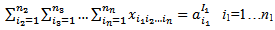
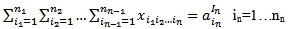
- The general n indexes transportation problem was first proposed by Ninh in 1979[16]. From this general problem, they have
 n index problems (nITP) according to the constrains on summation of
  indexes.[17]. Being different from the precedent thinking, Ninh did not use the n dimensional super box to solve it, he gave an exact method on the plan, an extension of potential method coordinating the resolution of the primal and dual problems. However, this result does not cover the solution of all particular problems of nITP because he proposed only the necessary condition and the sufficient condition so that the general problem has a solution[17]. Among these n index problems, Ninh decided to solve a particular case with the summation on (n-1) indexes which contributes significantly in economic terms. It is presented: Determine
  ij = 1…nj j = 1…n for
  | (6) |
 | (7) |
 | (8) |
 | (9) |
 For solving this problem, Ninh proposed an exact method, an extension of potential method, by coordinating the resolution of primal and dual problems. Ninh also presented and demonstrated the theorem of the necessary and sufficient condition so that the problem has had the solution (solution existence condition - SEC). This problem was also presented under the geometric form with the constraint on decomposable cost parameter. This is a k dimensional super box A in which the rth dimension A(r) is composed of nr segments. The section Ari is a super box with k-1 dimensions that is attached to the segment i of the edge Ari. It was solved by an approached method[22].
3.4. Four Indexes Transportation Problem Group
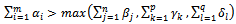
- Among these problems, the 4ITP is a model that concerns business organizations and attracts researchers. It fits the demands to the shuttle type in the companies that can use various trucks to transport goods from the manufacture (origin) to the deposit (destination). By replacing n=2 in the theorem SEC of n index problem, Ninh found the SEC for the 2ITP that existed previously. By replacing n=4, he obtained the SEC for the 4ITP as follow:Theorem 1: The necessary and sufficient condition so that the 4ITP has a solution:
 | (10) |
|
4. Resolution Method
- We found a sufficient condition so that the 4ITP is degenerated. Thus, we treat the non-validation of the SEC under the theoretical angle and the appearance of degeneration under the practical angle. By coupling with Ninh’s method[17], we present a general algorithm solving the 4ITP in all particular cases where the SEC is verified or not and the problem is degenerated or not.
4.1. Degeneration Condition
- We elaborate and demonstrate the sufficient condition so that the 4ITP is degenerated with a constraint where the SEC is verified.
4.1.1. General Form
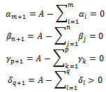
- Theorem 2: If there are
 ,
,  ,
,  , q1 values
  that:sum of these
  = sum of these
  sum of these
  = sum of these
  then, the 4ITP will be degenerated.We permute m1 equations whose right side are these
 , n1 equations whose right side are these
 , p1 equations whose right side are these
 , q1 equations whose right side are these
  at the first lines in each group. Thus, in order to simplify but not to diminish the generality of the problem, we present the sufficient condition under the reduced form.
4.1.2. Reduced Form
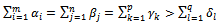
- Theorem 3: If there are numbers
 that:
that: 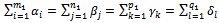 | (11) |
4.1.3. Demonstration
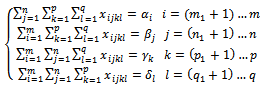
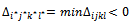
- We demonstrate the theorem for the reduced form. Suppose that the constraint system (2...5) responds to the theorem (3), we demonstrate that this problem is degenerated. Thus, it is only necessary to find a degenerated solution in order to demonstrate the degenerated 4ITP, i.e. the number of positive variables of this solution is less than (m+n+p+q-3).For this purpose, we seek a method to transform the initial problem into two sub-problems whose system of constraints are independent linear equation systems. We choose the variables
 to respond to the constraints:
 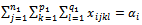 i = 1...m1This means that
  first origin nodes provide
  first goods types to
  first destination nodes by
  first vehicle types.We choose the variables
  to respond to the constraint:
  This means that
  last origin nodes provide
  last goods types to
  last destination nodes by
  last vehicle types. In order to it, we represent the constraints (2…5) as follow:
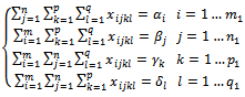 | (12) |
 | (13) |
 | (14) |
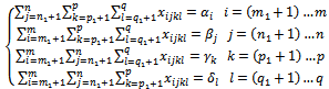 | (15) |
 for
for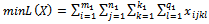 subject to:
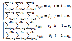 → The constraints system (14) of this problem responds to its SEC (the relationship 10). Therefore, we determine the maximum
  of positive variables. (condition 16)→ We determine the null variables that belong to the constraint system (12) but not belong to the constraint system (14). (condition 17)→ Thus, all of positive and null variables responding to the condition (16) and null variables responding to the condition (17) are the roots of the constraint system (12). The number of positive variables is maximum
  • For the sub-problem 2:Determine les variables
 for:
for: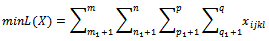 subject to:
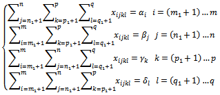 → From (10) and (11), we have:
 | (18) |
 of positive variables (condition 19).→ We determine the null variables that belong to the constraint system (13) but not belong to the constraint system (15) (condition 20).→ Thus, all of positive and null variables responding to the condition (19) and null variables responding to the condition (20) are the roots of the constraint system (13). The number of positive variables is maximum
  • For the initial problem:→ The set of variables
  of the systems (12) and (13) being determined above-mentioned responds to the constraints (2…5). So it is a solution for the 4ITP. → The number of positives variables
  of this solution is at most:

 .This solution is degenerated. Therefore, the initial problem is degenerated.
4.2. Degeneration, General Resolution Principle
- Based on the result of the sufficient condition so that the 4ITP is degenerated, we notice that the cause of degeneration of 4ITP can be defined as the transportation problem divided into two independent sub-problems and each sub-problem responds to the SEC. In order to eliminate the degeneration, we must modify the initial problem so that it cannot be divided into two independent sub-problems, i.e. each sub-problem does not respond to SEC. For this purpose, we add parameters at right side in the constraints of this problem so that each sub problem does not respond to the SEC but the initial transportation problem always responds to the SEC. Thus, the main idea of the resolution method is that we must add to the sub problem 1 and subtract from the sub problem 2 the same ε. We will at once add ε to the right side of one constraint equation that belongs to the group i of sub problem 1 and subtract ε from the right side of one constraint equation that belongs to the group i of sub problem 2. This means that the SEC is not cancelled. Thus, we demonstrate that after modifying the initial transportation problem, we obtain a new problem that can be solved and un-degenerated. However, in fact the research of numbers
 is relatively difficult even if we know they exist. Therefore, we propose a practical algorithm to recognize a degenerated problem and eliminate the degeneration for two cases: → Case 1: The degeneration appears in the elaboration process of the first solution → Case 2: The degeneration appears in the process of solution improvement to obtain the better solution.
4.3. Degeneration, Resolution Method (Case 1)
4.3.1. General Principle
- For the case 1, during the process of determining a variable xijkl>0 of the first solution, if we lose more than one equation in the constraints, the solution is degenerated. Supposing that we lose two equations in the constraints, there will be two equations of which value at right side becomes zero. To remove the degeneration, we keep the value zero on the right side of one equation and for the value zero on the right side of the other equation, we add ε (ε>0 and infinitesimal) and we simultaneously subtract ε from the right side of one equation that belongs to this group to respond to the SEC.We have four particular large groups for determining a first positive variable
 of the first solution. Among them, the first case illustrates an un-degenerated solution, the other cases illustrate the degeneration.
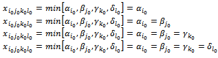
4.3.2. Method
- Suppose that we determine the variable
 .This variable represents only in the equations whose right side is
 . The equations are:
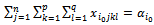 | (21) |
 | (22) |
 | (23) |
 | (24) |
4.3.2.1. Case 1
 The equation (21) is written:
  | (25) |
 Car
Car  the equation (25) becomes:
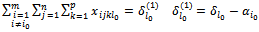
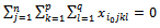 | (26) |

 , we have
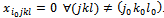 . Thus, we determine the variables
  and
and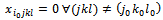 , and the constraint system (2...5) loses an equation. For the equation (22), it is written:
 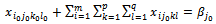 | (27) |
 Because
  and
and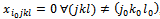 ,the equation (27) is written:
 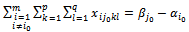 | (28) |
 , the equation (28) is written:
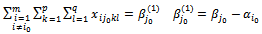 | (29) |
 | (30) |
 | (31) |
 We see that after determining the variables
  and, the new constraint system always responds to the SEC:
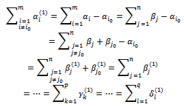 We continues determining the second variable, third variables,…until when we obtain the first solution.We similarly execute for the other cases:
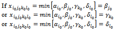
4.3.2.2. Case 2
 Similarly to case 1, we have:
  and
and 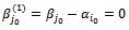 Thus, the constraint system (2…5) loses two equations, the solution obtained will be degenerated. To eliminate the degeneration, we keep:
  and we give:
  Thus, we must replace
  with
with  and
and  with
with  (with one
  so that the constraint system always responds to the SEC. We continue determining the second positive variable.
 4.3.2.3. Case 3
 Similarly to case 1, we have:
 and
and  Thus, the constraint system (2…5) loses three equations, the solution obtained will be degenerated. To eliminate the degeneration, we keep:
  and we give:
 Thus, we must replace:
  with
with 
 with
with  In order that the constraint system always responds to the SEC, we must replace:
  We continue determining the second positive variable.
4.3.2.4. Case 4
 Similarly to case 1, we have:
  Thus, the constraint system (2…5) loses four equations, the solution obtained will be degenerated. To eliminate the degeneration, we keep:
  and we give:
 Thus, we must replace:
  with
with 
 In order that the constraint system always responds to SEC, we must replace:
  We continue determining the second positive variable.Thus, once we determine a positive variable, the constraint system (2…5) loses an equation and continue...., finally, we obtain a solution that consists of (m+n+p+q-3) positive variables. This is the solution un-degenerated.
 4.4. Degeneration, Resolution Method (Case 2)
4.4.1. General Principle
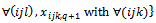
- The transformation process of an un-optimal solution for searching a better solution is presented as follows: → Determine the parameters:
 with all xijkl > 0
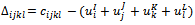 with all xijkl = 0If
  Δijkl ≥ 0, the solution is optimal. If
  Δijkl < 0, the solution is not optimal. We must execute the next steps: → Determine
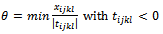
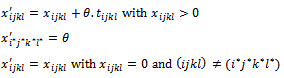
 Suppose that
 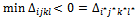 → Determine the parameters tijkl corresponding to the variables xijkl > 0 for:
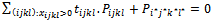 Pijkl is the coefficient vector of variables xijkl in the constraint system (2…5). It is the column vector with four digits 1 at the line i, m+j, m+n+k, m+n+p+l, the others are zero. → Determine:
  with tijkl < 0 and suppose that
 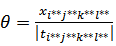 → Elaborate the new solution:
 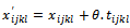 with
with 

 with
with  et
et 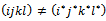 And we see that:
 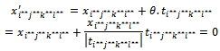 The new solution X’ has maximum (m+n+p+q-3) positive variables.Supposing that during this transformation process, we find a solution with two variables
  that are determined from positive variables (xijkl>0) becoming zero. This means that the number of positive variables xijkl of this solution is less than (m+n+p+q-3). It is a degenerated solution. To eliminate the degeneration, we add ε (ε>0 and infinitesimal) in the second variable zero. Thus, the SEC always fits but the amount of four members αi, βj, γk, δl is increased by ε. In mathematical term, the new transportation problem is different from the initial one because the total amount of transported goods increases more ε.
 4.4.2. Method
- For example, suppose that
 is the second variable becoming zero in the solution improvement process. → We give
  (ε>0 and infinitesimal)→ Because the variable
  represents in the equations whose right side is
 , we have:The right side
  must become
  The right side
  must become
  The right side
  must become
  The right side
  must become
  In the case there are more than two variables xijkl=0, we add ε1, ε2… to these variables based on the above principle to eliminate the degeneration. After obtaining the optimal solution, we replace all these ε with zero and we obtain the result for the initial 4ITP.
4.5. SEC not Verified, Resolution Method
4.5.1. General Principle
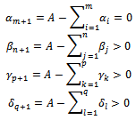
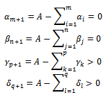
- If the transportation problem does not respond to the SEC, it is impossible to solve a transportation problem. Thus, we modify this problem to create a new problem coming up to our expectation. The modification principle is to add fictitious nodes and parameters (fictitious node m+1; fictitious node n+1; fictitious parameter p+1; fictitious parameter q+1) to create equality between the four amounts. The transportation cost is considered as null: from a fictitious node to all destination nodes, from all origin nodes to a fictitious destination node, to transport the fictitious goods or by using a fictitious vehicle. Note that:
 → For the index i: We add the node m+1 and note:
 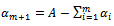 → For the index j:We add the node n+1 and note:
 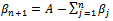 → For the index k:We add the parameter p+1 and note:
 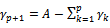 → For the index l:We add the parameter q+1 and note:
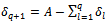
4.5.2. Method
- Based on this principle, we elaborate the new problem according to three main particular cases.
4.5.2.1. Case 1: An Amount in the Relationship (10) is Superior to Other
- E.g.
 Note
Note  We have
 The initial problem becomes:Determine the variables
  i=1...m, j=1...(n+1), k=1...(p+1), l=1...(q+1) for
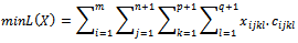 subject to:
 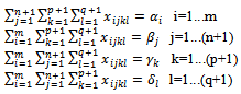 The SEC:
 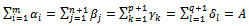 So the SEC is verified. The new problem is solvable.
 4.5.2.2. Case 2: Two Amounts in the Relationship (10) are Equal and Superior to Other
- E.g.
 Note
Note  We have
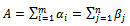
 The initial problem becomes:Determine the variables
  i=1...m, j=1...n, k=1...(p+1), l=1...(q+1) for
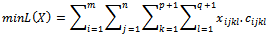 subject to:
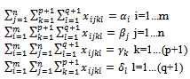 The SEC:
 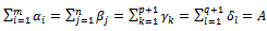 So the SEC is verified. The new problem is solvable.
 4.5.2.3. Case 3: Three Amounts in the Relationship (10) are Equal and Superior to the Last
- E.g.
 Note
Note  We have
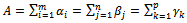
 The initial problem becomes:Determine the variables
  i=1...m, j=1...n, k=1...p, l=1...(q+1) for
 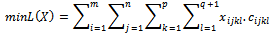 subject to:
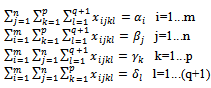 The SEC:
  So the SEC is verified. The new problem is solvable.
4.5.3. Fictive Variable Elimination
4.5.3.1. Elimination Principle
- We have four main groups of fictive variables corresponding to four fictive parameters: m+1, n+1, p+1, q+1.
 is the variables of the found optimal solution. We give: →
 for all j, k, l if
  . Contrary,
  ⇒ there are not the variables
  ⇒ this leads to having no variable
  →
→ for all i, k, l if
  . Contrary,
  ⇒ there are not the variables
  ⇒ no variables
  →
→ for all i, j, l if
  . Contrary,
  ⇒ there are not the variables
  ⇒ no variables
  →
→ for all i, j, k if
  . Contrary,
  ⇒ there are not the variables
  ⇒ no variables
4.5.3.2. Economical Signification
- The origin node (m+1), the destination node (n+1), the goods type parameter (p+1) and the vehicle type parameter (q+1) are fictives and are added in the constraint system so that the new transportation problem responds to the SEC. Thus, if we use:→ the goods quantity at the origin (m+1) to respond to the command of customer system, i.e. actually, we do not carry anything because this origin does not exist →the transportation cost for carrying the goods from this node must be equal to zero.→ the destination node (n+1) does not actually exist, i.e. there is not any order at the node (n+1) → the transportation cost for shipping the goods to this node must be equal to zero.→ the goods type (p+1) does not actually exist →the transportation cost for shipping this goods type must be equal to zero.→ the vehicle type (q+1) does not actually exist → there is not the transportation cost corresponding to this vehicle type → the transportation cost is equal to zero.In the found optimal solution, if there are the variables with the fictive indexes, suppose that
 tons, we must give
  to obtain the reel variables in the optimal solution of the initial problem. Theoretically, this elimination means that these four tons of goods type 4 are shipped from the origin node(m+1) to the destination node 5 by the truck type 7 but actually, the truck type 7 is under four tons loaded or this truck is not filled.
 4.6. General Resolution Algorithm, Real Variables
- There are two main cases: → If the 4ITP is not degenerated and the SEC is verified, we use Ninh’s method[17]→ If not, our method will be used to transform the problem in the first case. The steps of our general algorithm solving the 4ITP in all particular cases are presented as follow:
4.6.1. Step 1(Test the SEC)
- We test the SEC (the relationship 10)→ If yes then go to the step 3→ else go to the step 2
4.6.2. Step 2 (Transform the initial problem)
- Search
 Supposing that
  Add a fictitious origin node (m+1) with the quantity is
  .Give
.Give 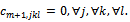 Similarly, execute for any amount that is less than A to obtain the relationship
 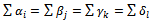 Go to the step 3.
4.6.3. Step 3(Search the first solution)
4.6.3.1. Loop 1 (Search the first variable)
- Determine
 ◆ If
◆ If 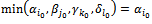 Give
Give  Thus,
Thus,  with
with 
 The right part in the constraints becomes:
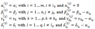 ◆ If
◆ If 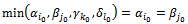 Replace
  with
with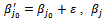 with
with  with one
  ◆ If
◆ If 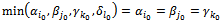 Replace
  with
with  with
with  with one
  Replace
  with
with with
with  with one
  ◆ If
◆ If  Replace
  with
with  with
with  with one
  Replace
  with
with 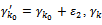 with
with  with one
 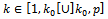 Replace
  with
with 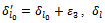 with
with  with one
 Thus, with
  we have the relationship
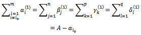 We similarly execute to the other cases.Go to the loop 2 to determine the next variable.
4.6.3.2. Loop 2 (Search the next variable)
- Determine
 Return to the loop 1. When all the right sides of the constraint systems (2...5) are equal to zero, stop the loop. We obtain the first solution. Go to the step 4. Remarking that the variables
 will be determined in the final sequence. .
 4.6.4. Step 4 (Control the optimality of the solution X)
4.6.4.1. Determine the Potentials 
- Determine the potentials


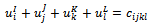
4.6.4.2. Compute the Elements 
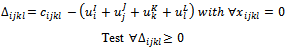 | (32) |
4.6.5. Step 5 (Modify the solution X to find the other better solution)
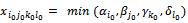
4.6.5.1. Determine the Element 
- Determine the element
 If there are several
  that get the minimum value, give any
  of these
 .Determine the element
  for
for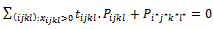 The right part of this constraint is the vector 0.
 is the coefficient vector of variables xijkl in the constraint. It is the column vector which has four digits 1 at the line i, m+j, m+n+k, m+n+p+l, the others are zero.
4.6.5.2. Elaborate a New Solution
- Determine θ for
 We test, among these found variables
  that are calculated from
 , there is just one being zero.→ If yes then the solution is un-degenerated.→ else keep the value 0 of a variable and suppose that the value 0 of the others are respectively
  Return to the step 4.
4.6.6. Step 6 (Find the optimal solution of the initial problem)
- → Replace ε with zero in the found variables.→ Remove the variables that correspond to the fictitious nodes added and the fictitious parameters in the step 2.Finally, we obtain the optimal solution of the initial problem.
5. Results
5.1. 4ITP, Numerical Examples
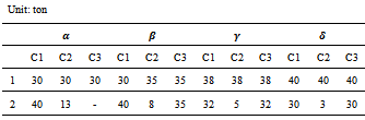
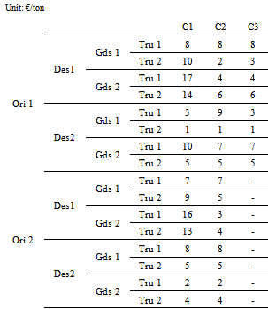
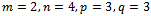
- Based on the resolution method in the exact angle, we give numerical examples on small artificial database. The aim of this section is to test the method before an implementation in industry. We examine three cases:Case 1: SEC is satisfied and the degeneration appears in the first solution.Case 2: SEC is satisfied and the degeneration appears on the solutions modification process. Case 3: SEC is not satisfied. In this simple example, the hypothesis is composed of 8 parameters, 16 unit costs and 16 variables for case 1 and 2; 7 parameters, 8 unit costs and 8 variables for case 3. The table 2 shows the parameters of the origins, destinations, the types of goods and the types of trucks. The table 3 presents the unit transportation cost. Specially, in the case 3, because of the weakness of the origin 2, all unit transportation costs for goods that are left at the origin 2 are considered as null.
|
|
|
|
5.2. 4ITP, Optimal Planning
|
5.3. 4ITP, Performances
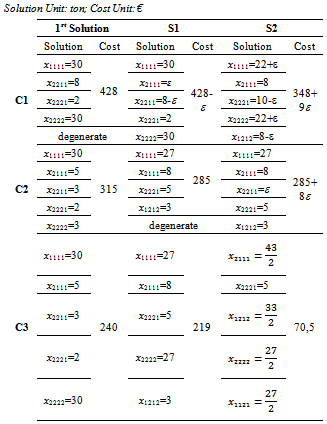
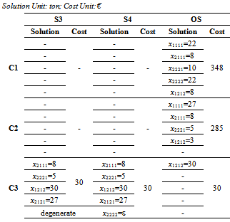
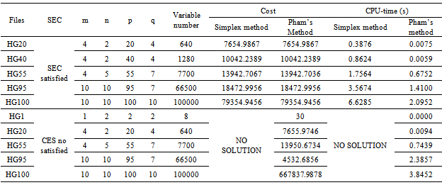
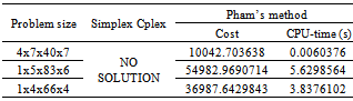
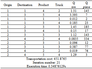
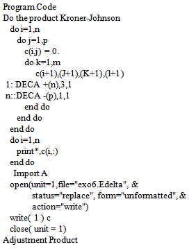
- Our algorithm (or Pham’s method) is programmed in Fortran 95 language with Gfortran compiler running on a computer equipped with a CPU Intel Core 2 at 1,97Ghz. To test two methods (our method and simplex method), we use the real series which are not degenerated and they are divided into two groups: SEC is verified and SEC it not verified.The table 7 presents some performances of our program with real variables: → In the case of SEC verified, both methods get the optimal value of the objective function: the minimum transportation cost. However, the execution time of Pham’s method is fast enough to handle middle sized problems and large ones. It treats up to 100,000 variables in 2 seconds compared to 6.6 seconds for the simplex method. → In the case where the SEC is not satisfied, Pham’s method always gets the optimal solution and the execution time is very fast. It treats up to 100,000 variables in 3.8 seconds while the simplex method stops immediately without solution. We found the degeneration series and tested them by two methods: Pham’s method and simplex method. The table 8 presents an extract of the execution results by both methods for the degeneration series with the condition of SEC verified. The simplex and its options in Cplex cannot avoid the degeneration for all cases in the 4ITP resolution field. The numerical results show that, for the case where the simplex method cannot find the optimal solution, Pham’s method eliminated the degeneration and easily obtained the optimal solution.
|
|
5.4. 4ITP, Extension on Integer and Mix Variables
- Building on the foundation of resolution method for 4ITP, we treat the integer model by using the elements in FORTRAN 95 library. We also develop a program coupled with the main program of the initial problem. The table 8 illustrates our method on the data of a simple model with
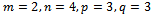 and the SEC is not satisfied.
|
 and the SEC is not satisfied.
|
|
6. Implementation
- In this section, we present work in progress. From the industrial database, we develop an algorithm to determine the input database for the model 4ITP. This is implementing in the logistics management system of Airbus’s subcontractor in France.
6.1. Industrial Case Study
- The Hitchcock’s problem was elaborated by the request of the Aéropostale de nuit company and fully resolved in the 50’s of last century. Currently, there are at least three companies in France using Hitchcock model in their logistics system. These are leading groups in the field of mass transport: Fedex, Aéropostale de nuit and Air-France cargo. These companies must deliver several types of goods and often use several vehicle types. Therefore, Fedex applies Hitchcock model by using an approximate model to unify all types of product in one common product type and all vehicle types in one common type.
 | Figure 2. Order and delivery system (AAS and Airbus) |
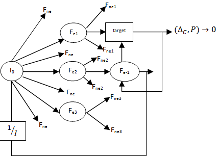
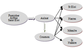 | Figure 3. AAS transportation diagram |
6.2. Industrial Database
- → AAS consists of m production sites Oi (i=1…m).→ They manufacture p product types Sk (k=1…p).→ The production capacity of site Oi for the product type Sk in period t is
 (ton).→ At the site Oi, the quantity of product type Sk in inventory at the end of period t-1 is
  (ton).→ At the site Oi, the average unit cost for storing a unit of product type Sk in period t is cki (€/ton).→ This group consists of q vehicle types Hl (l=1…q) to deliver goods to its customers. The load of vehicle type Hl is
  (ton).→ These products are delivered to the customer, Airbus Industry. It has a production network that consists of r manufacturing sites Db (b=1…r). → The demand of site Db for the product type Sk in period t is
  (ton).→ The raw materials are stored in a logistics network of n warehouses Dj (j=1…n). The storage capacity of Dj in period t is
  (ton).→ The average unit cost for transporting a unit of goods type Sk from origin Oi to destination Dj by vehicle type Hl in period t is cijkl (€/ton).
6.3. Database of 4ITP model
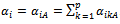
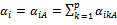
- The steps are performed to determine the parameters alpha, beta, gamma and delta of model as follow:Step 1: Calculate the parameter
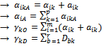 Step 2: Determine
  and
and  → Case 1: If
  we give
 . Go to the step 4.→ Case 2: If
  we give
 . Go to the step 4.→ Case 3: If
  we give
  It means that we adjust
  of manufacturer to
  of customer. Go to the step 3.Step 3: Adjustment If we adjust
  of manufacturer to
  of customer, i.e. we reduce the total quantity of product type Sk at the manufacturer so that it is equal to the quantity of this type at the customer. This leads to reducing the total delivery quantity of manufacturer. So the following questions must be answered: which production site will stock the surplus quantity of product Sk and how many tons? The aim is to avoid delivering the goods on surplus to customers.We adjust
  to
to  by using the ant colony algorithm, an extension of PSO method (particle swarm optimization).→ The general principle of adjustment method is presented in the section 6.4.→ The criterion of adjustment:● minimize the total average storage cost at all production sites in period t. ● product type k: total offer = total demand.After adjusting, we obtain
  (It should obtain that
 ). Go to the step 4.Step 4: Determine the parameters of 4ITP model→ Offer at origin: Delivery capacity =
  → Demand at destination: Storage capacity (known in the industrial database) =
  → Goods types: the quantity of product type Sk =
  → Vehicle types: load vehicle type Hl (known in the industrial database) =
6.4. Adjustment Method
- The adjustment method is based on the principle of the ant movement to build new solutions and determine the vectors carrying adjustment variables. Each ant builds a solution from the origin node by choosing isomorphic arcs to probabilistically un-fuzzy treat. In an arc, it typically selects the next arc by using wefts (line from origin to destination) or capacity direction arcs C-i. The “blind” choices are needed to explore new solutions and determine costs. In fact, the ant is blind with a probability of selected iteration, then j is chosen randomly among the k closest arcs that remain to be treated. With the probability 1-pr, we consider the chosen paths as well as direction. This last formula is classic and at the same time, it considers the visibilities of arcs and wefts weighted by chosen powers.
 | Figure 4. General principle of parameter adjustment method by ant colony algorithm |
6.5. Result
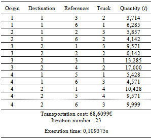
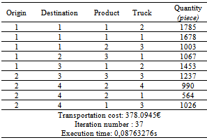
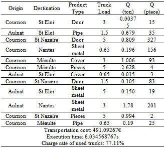
- From the real industrial database provided by AAS, we use the algorithm to determine the input data of 4ITP model. Then, we use the mixed model to determine the optimal transportation schedule. An extract of an optimal transportation planning for the week 12/2012 is presented in the table 12. This is the first results of the implementation process.
|
7. Conclusions
- Our work has resulted from the resolution of all previously untreated cases of 4ITP under exact mathematical angle. In the domain of transportation problem, a particular case of linear programming, our method takes more advantages over the simplex. Indeed, the simplex stops immediately without solution in the case where the problem is degenerated and (or) the SEC is not verified. Our method (Pham’s method) directly eliminates the degeneration in the same iteration, the execution time is fast (three times as fast as the simplex) and the obtained solution is optimal. Thus, we have proposed a mathematical tool for solving optimization problem of weight transportation. In operational angle, we obtain the first results in implementation process. We foresee to develop transportation management software user-friendly interface that allows the logistician to entry ordered items. This will be coupled with GPAO, production software of AAS’s enterprise, which automatically receives the ended reference markers. Thus, before making the delivery of parts, the logistics management will interrogate this management software that edits a delivery plan after optimization. This plan includes the number of used trucks for a list of part from origins to destinations.