2000 Mathematical Classification 90Bxx, 90 B05

1. Introduction

Kaleidoscopic pattern of inventory control system with deterioration is much more difficult to be investigated by the researchers engaged in the field. In its investigative design and framework, mathematical ideas have exceedingly shown well for dwelling upon the concern of inventory control system with aforesaid pattern of inventory. Deterioration of inventory encompasses commodities such as such as foods, vegetable, drugs, pharmaceuticals, medicine, gasoline, blood and radioactive substances deterioration takes place during the normal storage period of the units. As a result, while determining the optimal inventory policy of that type of products, the loss due to deterioration cannot be ignored.

In the literature of inventory theory, the deteriorating inventory models have been continually modified so as to accumulate more practical features of the real inventory systems. A number of authors have discussed inventory models for non deteriorating items. However, there are certain substances in which deterioration plays an important role and items cannot be stored for a long time. When the items of the commodity are kept in stock as an inventory for fulfilling the future demand, there may be the deterioration of items in the inventory system. Various types of inventory models for items deteriorating at a constant rate were discussed by[1],[2],[3] and[4] etc.In practice it can be observed that constant rate of deterioration occurs rarely. Most of the items deteriorate fast as the time passes. Therefore, it is much more realistic to consider the variable deterioration rate. In a realistic product life cycle, demand is increasing with time during the growth phase.[5] investigated an inventory system with power demand pattern for items with variable rate of deterioration. [6] studied the inventory system with two-parameter exponential distributed hazardous items in which production and demand rate were constant.[7] considered an EOQ model in which inventory is depleted not only by demand, but also by deterioration at a Weibull distributed rate, assuming the demand rate with a ramp type function of time.

[8] developed an inventory model for a deteriorating item having an instantaneous supply, a quadratic time-varying demand and shortages in inventory. They had taken a two-parameter Weibull distribution to represent the time to deterioration.[9] considered an inventory model for deteriorating items in which demand increases with respect to time, deterioration rate, inventory holding cost and ordering cost are all continuous functions of time. Shortages are completely backlogged. The planning horizon is finite.

[10] formulated an order-level lot-size inventory model for a time-dependent deterioration and exponentially declining demand.[11] reviewed the recent studies about the deteriorating items inventory management research status. They provided a comprehensive introduction, compared with the extant reviews and proposed some key factors which should be considered in the deteriorating inventory studies. This survey provides a clear overview of the deteriorating inventory study field, which can be used as a starting point for further study.

A key assumption of the basic EOQ model is that stock outs are not permitted. Relaxing the basic EOQ that stock outs are not permitted led to the development of EOQ model for the two basic stock out cases: backorders and lost sales. What took longer to develop was a model that recognized that, while some customers are willing to wait for delivery, others are not. Either these customers will cancel their orders or the supplier will have to fill them within the normal delivery time by using more expensive supply methods. While there have been a number of models developed for the EOQ model with partial backordering, most of them incorporate considerably more complicated assumption sets than the classic EOQ model do. Furthermore, when the shortage occurs, some customers are willing to wait for back order and others would turn to buy from other sellers.

[12] developed economic order quantity models that focused on deteriorating items having a deterministic demand pattern with a linear trend and shortages. They assumed that the inventory deteriorates over time at a constant rate. The inventory replenishment policy was considered over a finite time-horizon.[13] considered an inventory model for items with Weibull distributed deterioration. They assumed that the demand rate is a power function of time and allowed for shortages.[14] considered the variable lead-time EPQ model with shortages. He presented a new approach, without reference to the use of derivatives but with algebraic derivation, to solve the deterministic EOQ models with/without shortages.

[15] developed an inventory model with ramp type demand, starting with shortage and three – parameter Weibull distribution deterioration.[16] developed an inventory model with linear demand rate. Shortages in the inventory are allowed and were completely backlogged. They had assumed that the production rate is finite and proportional to the demand rate.[17] developing an inventory model with time dependent Weibull demand rate where shortages are allowed and are completely backlogged. The production rate is assumed to be finite and proportional to the demand rate.

[18] developed an order level inventory system for time dependent linearly deteriorating items with decreasing demand rate. They assumed that the demand rate is time dependent and developed two EOQ models for without shortage case and with shortage case.[19] considered the production inventory problem in which the deterioration is Weibull distribution, production and demand are quadratic function of time. Shortages of cycle are allowed in the inventory system.

Researchers such as[20],[21] and[22] considered the constant partial backlogging rates during the shortage period in their inventory models. In many cases customers are conditioned to a shipping delay and may be willing to wait for a short time in order to get their first choice. In some inventory systems, such as fashionable commodities, the length of the waiting time for the next replenishment would determine whether the backlogging will be accepted or not. Therefore, the backlogging rate should be variable and dependent on the length of the waiting time for the next replenishment. When a stock out situation occurs, only a fraction of demand occurring at a given time is backordered. And that fraction is a decreasing function of the waiting time. The approach given is revenue based and does not require specifying the backorder cost or lost sale cost which is very difficult to estimate in reality.

[23] investigated optimal lot sizing for an EOQ model under conditions of perishability allowing shortage and partial backlogging. He modelled the backlogging phenomenon using a new approach in which customers are considered impatient.[24] suggested a continuous review inventory model over a finite-planning horizon with deterministic varying demand and constant deterioration rate. The model allows for shortages, which are partially backlogged at a rate which varies exponentially with time. They established an optimal replenishment policy.[25] developed the deterministic EPQ model with partial backordering when a percentage of stock outs will be backordered.

Many researchers have modified inventory policies for deteriorating items by considering the time proportional partial backlogging rate such as[26],[27],[28],[29],[30],[31], [32] and so on.[33] extended model of[13] by proposing a general class time-proportional backlogging rate to make the theory more complete and provided the necessary condition to find the optimal solution.[34] proposed an EOQ inventory mathematical model for deteriorating items with exponentially decreasing demand. In the model, the shortages are allowed and partially backordered. They show that the minimized objective cost function is jointly convex and derive the optimal solution.

[35] described an EOQ model with time-varying deterioration, partial backlogging which depends on the length of the waiting time for the next replenishment, linearly time-varying demand function over a finite time horizon and variable replenishment cycle.[36] developed a deterministic inventory model for infinite time-horizon incorporating partial backlogging and decrease in demand. Demand at any instant depends linearly on the on-hand inventory level at that instant. Deterioration of items begins after a certain time from the instant of their arrival in stock.[37] studied a deterministic inventory model for deteriorating items under time-dependent partial backlogging and proved that the optimal replenishment solution not only exists but is also unique.

[38] considered an EOQ model for deteriorating items with exponential time varying demand. They assumed that the backlogging rate is dependent on the length of the waiting time for the next replenishment.[39] presented an optimization framework to derive optimal replenishment policy for perishable items with stock dependent demand rate. The demand rate is assumed to be a function of current level inventory and the inventory deteriorates per unit time with variable deterioration rate. The shortages are allowed and partially backlogged with a variable rate, which depends on the duration of waiting time up to arrival of next lot.[40] developed a single item perishable inventory model assuming that the demand is time dependent accelerated growth-effect of accelerated growth-steady type. The deterioration of inventory starts after a certain time. Shortages are allowed and are partially backlogged.

[41] considered a deterministic inventory model in which items are subject to constant deterioration and shortages are allowed. The unsatisfied demand is backlogged which is a function of time.[42] considered an order level inventory model for seasonable/fashionable products subject to ramp type demand rate. The unsatisfied demand is partially backlogged with a time dependent backlogging rate. In addition, the product deteriorates with a time dependent deterioration rate.[43] developed a deterministic inventory model for deteriorating items in which shortages are allowed and partially backlogged. Recently, authors[44],[45] and[46] have attempted computational approach to various inventory models and discussed their applications.

[47] developed a partial backlogging inventory model. They proposed the prediction method and algorithms for ordering period as well as for minimum total cost.[48] presented Economic Production Lot Size model with constant deterioration. Shortages are permitted in inventory with partial backlogging.[49] described an EOQ model for a deteriorating item considering general time-dependent demand, time-dependent partial backlogging over a finite time horizon and variable replenishment cycle.[50] developed an inventory model with time dependent two-parameter Weibull demand rate whose deterioration rate increases with time. Each cycle has shortages, which have been partially backlogged.

There are a number of situations in which a customers or vendors of some sort are assumed to receive the demand in bulk of inventory are subject to put in queue at a service facility. The goal of queuing is essentially to trade-off the cost of providing a level of service capacity and the customers waiting for service.

With this motivation, in the present paper an attempt is made to formulate a partial backlogging inventory model by incorporating the deterioration effect and time-dependent power pattern demand rate. Deterioration of items begins after a certain time from the instant of their arrival in stock, we name it as life time of items, and deterioration rate is a quadratic function of time. Unsatisfied demand is partially backlogged with a variable rate. To suit present day competition in the market, the backlogging rate is inversely proportional to the duration of waiting time up to arrival of next lot. The differential equations are derived and the instantaneous state of inventory is obtained analytically. The total cost function, which consists of setup cost, holding cost, backordering cost, lost sale cost, deterioration cost, waiting cost and procurement cost is constructed and subjected to the optimization which in turn gives us the system of non linear equations. Further, a computing algorithm is proposed to find the solution of the system by using the N-R method. We compute the optimal inventory period and total optimal average cost as most important performance measures for the model. Numerical demonstration and sensitivity analysis have been carried out for the model to identify the most sensibilities of various parameters involved in the system leading to interesting observations which seem to be consistent with its economic insights. This model is much useful for analysing the planning of the seasonal and fashionable products with the notion of decay or obsolete.

2. Assumptions and Notations

In this paper we have made the following notations and assumptions in the formulation of proposed mathematical model of the inventory system.

2.1. Notations

I (t) : the inventory level at any time t, t ≥ 0.

S : the initial inventory level.

μ : the life time of items.

: the average arrival rate.

: the average service rate.

L_S : the number of customers waiting for inventory.

C_O : the set up cost for each replenishment.

C_H : inventory holding cost per unit time.

C_D : deterioration cost per unit.

C_S : shortage cost for backlogged items.

C_L : the unit cost of lost sales.

C_W : waiting cost per customer per unit time.

C_P : procurement cost.

T : the planning horizon.

TAC (t₁) : the total average cost.

2.2. Assumptions

I. A single item is considered over the fixed period T units of time.

II. Customers are waiting in line for getting inventory items. They arrive on a precise schedule (deterministic) of evenly spaced intervals and service process is well scheduled.

III. and are assumed to be constant and are related by

IV. Deterioration of the items takes place after the life time of items.

V. The variable deterioration rate θ(t) is time dependent quadratic function such that θ(t) = θt², 0<θ<<1.

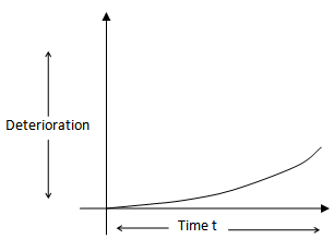Figure 1. Deterioration-time relationship

VI. There is no replenishment or repair of deteriorated items during a given cycle.

VII. The replenishment occurs instantaneously at an infinite rate.

VIII. Lead time is negligible.

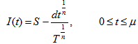
IX. The demand rate is D(t) at any time t such that, where d is the fixed quantity, n is the parameter of power demand pattern, the value of n may be any positive number.

X. Shortages are allowed and backlogging rate is , when inventory is in shortage. The backlogging parameter k is positive constant and 0XI. All of the cost parameters are positive constants.

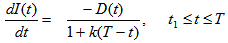
3. Mathematical Model

3.1. Model Formulation and Solution

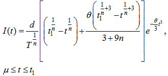
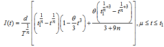
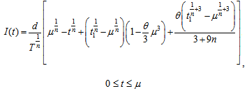
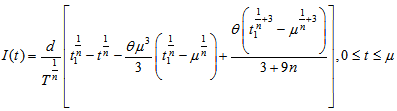
Let us assume that Q be the total amount of inventory produced or purchased at the beginning of each cycle. After fulfilling the backorders let we get an amount S (>0) as initial inventory. During the period (0, μ) the inventory level gradually decreases due to market demand only. After life time deterioration can take place, therefore during the period (μ, t₁) the inventory level gradually abates due to market demand and deterioration of items and falls to zero at time t₁. Shortages take place in the periods (t₁, T) which are partially backlogged. The depletion of inventory level is shown in the following figure.

The differential equations governing the inventory level at any time t during the cycle (0, T ) are given as following,

(3.1)

(3.2)

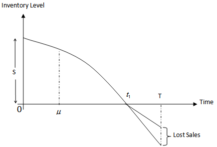Figure 2. Partial Backlogging Inventory Model

(3.3)

The solution of equation (3.1) is

(3.4)

Taking the first two terms of the exponential series and then integrating we get the solution of equation (3.2) as

(3.5)

Now taking the first two terms of the exponential series and neglecting the term containing α² the equation (3.5) becomes

(3.6)

Similarly the solution of equation (5.3) is

(3.7)

From equation (3.5) and (3.6), we have

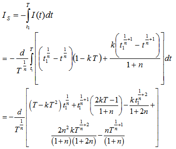
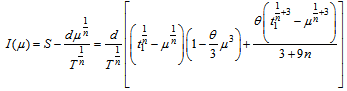So that, the value of initial inventory level (S) is given by

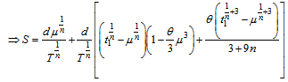(3.8)

Using equation (3.8) in equation (3.5) we get

(3.9)

During period (0, T ) total number of units holding I_H is

Using equation (3.9) and equation (3.6) we get

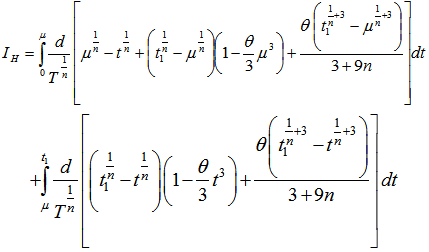Calculating further we get

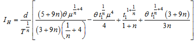(3.10)

Total amount of deteriorated items I_D, during the period (0, T ) is

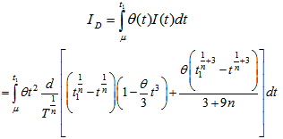Integrating this, neglecting the term containing θ² or higher degree of it as

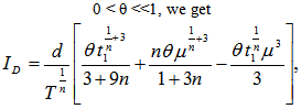(3.11)

Total amount of shortage units I_S during the period (0,T ) is given as

(3.12)

Total amount of lost sales I_L during the period (0, T ) is given by

(3.13)

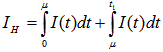
3.2. Cost Analysis and Optimization

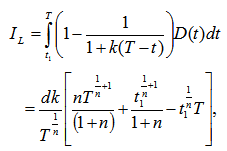
The total waiting cost for the customers in the system _.

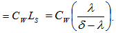Total average cost of the system per unit time is given by

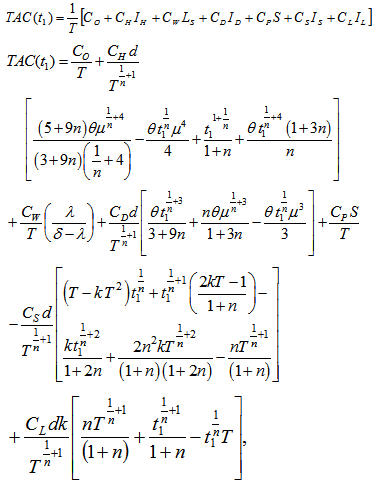(3.14)

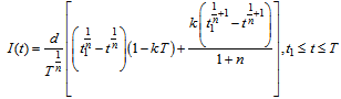
To minimize total average cost per unit time , the optimal value of t₁ can be obtained by solving the following equation

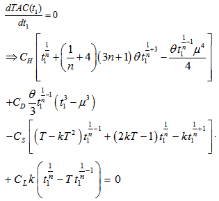(3.15)

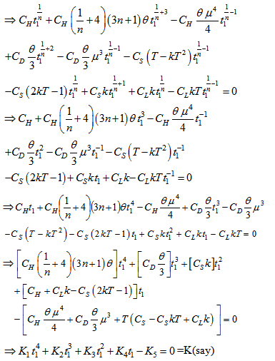(3.16)

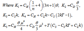Equation (3.16) is a non-linear equation in t₁ and its value is obtained by using N-R method and following algorithm by using C++ provided total cost is minimum and its second derivative is positive for being t₁ optimal. The following value of second derivative in (3.17) is tested true after required parameters are computed

(3.17)

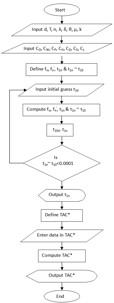Figure 3. Computing Algorithm

After substituting the optimal value of t₁ in the expressions of initial inventory level (3.8) and minimum total average cost per unit time are computed finally as optimal.

3.3. Computing Algorithm

Following computing algorithm is developed to find out the optimal inventory period and total optimal average cost of the inventory system.

4. Sensitivity Analysis

4.1. Numerical Example

We have considered the following parameter values to illustrate the model numerically. =1000 units, =Rs. 500 per order, =5, =4, =Rs. 35 per unit per year, =100 per unit, =Rs. 80 per unit per year, =Rs. 20 per unit, =1 year, =4 units, =10, =8, =0.01 unit, =0.3 year, =0.15 unit. Then to minimize the total average cost, optimal values of the decision variables are obtained as =0.766271 year, =1000.108444 units, =Rs. 6933.95 per year.

4.2. Tables, Graphics and Observations

The aim of the sensitivity analysis is to demonstrate the variability of the model based on the simulations or the hypothetical data-input. In this chapter, we prefer the hypothetical data-input to run the search program of the system. It is the process of varying model parameters over a reasonable range and observing the relative changes in the model response. Remarkable are the observed changes in the optimal cycle time and total optimal average cost of the system.

We wrote a program in C++ to apply a one-variable version of N-R method to compute the optimal cycle time and consequently the total optimal average cost of the system is also computed. In sensitivity analysis, variational effect of parameters on the total optimal average cost is presented.

Table 1. Demand Coefficient d Vs. Optimal Total Average Cost (TAC*)       Demand Coefficient(d) % Change Inventory Period (t1*) Initial Inventory Level (S) Optimal Total Average Cost (TAC*) 500 -50 0.766271 500.05 3704.48 700 -30 0.766271 700.08 4996.25 900 -10 0.766271 900.10 6288.06 1000 0 0.766271 1000.11 6933.95 1100 10 0.766271 1100.12 7579.85 1300 30 0.766271 1300.14 8871.64 1500 50 0.766271 1500.16 10163.42

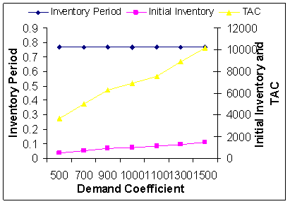Figure 4. Demand Coefficient d Vs. Optimal Total Average Cost

In Table and Figure 4, we observe that as demand coefficient increases, the optimal inventory period shows a negligible increment, while optimal initial inventory level as well as optimal total average cost shows significant increment. In fact, about 10% increase in demand coefficient amounts to approx. 0.04%, 10% and 9.32% increase in optimal inventory period, optimal initial inventory level and optimal total average cost respectively. Moreover, demand coefficient shows a positive correlation with optimal inventory period, optimal initial inventory level and optimal total average cost.

Table 2. Setup Cost       Vs. Optimal Total Average Cost (TAC*)             Setup Cost (CO) % Change Inventory Period (t1*) Initial Inventory Level (S) Optimal Total Average Cost (TAC*) 200 -60 0.766271 1000.108444 6633.95 300 -40 0.766271 1000.108444 6733.95 400 -20 0.766271 1000.108444 6833.95 500 0 0.766271 1000.108444 6933.95 600 20 0.766271 1000.108444 7033.95 700 40 0.766271 1000.108444 7133.95 800 60 0.766271 1000.108444 7233.95

In Table and Figure 5, we find that as setup cost increases, almost the optimal inventory period and optimal initial inventory level show non-significant increase whereas optimal total average cost increases significantly. Numerically, about 20% increase in setup cost causes about approx. 0.02%, 0.03% and 1.44% increase in optimal inventory period, optimal initial inventory level and optimal total average cost respectively. Thus, setup cost shows a positive correlation with optimal inventory period, optimal initial inventory level and optimal total average cost.

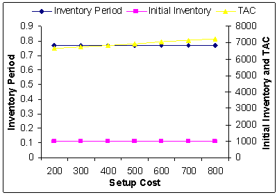Figure 5. Setup Cost Vs. Optimal Total Average Cost (TAC*)

Table 3. Waiting Cost       Vs. Optimal Total Average Cost (TAC*)       Waiting Cost (CW) % Change Inventory Period (t1*) Initial Inventory Level (S) Optimal Total Average Cost (TAC*) 2 -60 0.766271 1000.108444 6948.95 3 -40 0.766271 1000.108444 6943.95 4 -20 0.766271 1000.108444 6938.95 5 0 0.766271 1000.108444 6933.95 6 20 0.766271 1000.108444 6928.95 7 40 0.766271 1000.108444 6923.95 8 60 0.766271 1000.108444 6918.95

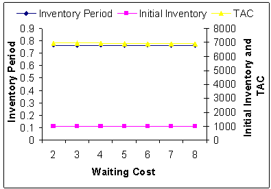Figure 6. Waiting Cost Vs. Optimal Total Average Cost (TAC*)

In Table and Figure 6, we find that as waiting cost increases, the optimal total average cost decreases. Numerically about 20% increase in waiting cost creates about % increase in optimal total average cost. Moreover, waiting cost shows a negative correlation with optimal total average cost.

Table 4. Procurement Cost (Cp) Vs. Optimal Total Average Cost (TAC*)       Procurement Cost (Cp) % Change Inventory Period (t1*) Initial Inventory Level (S) Optimal Total Average Cost (TAC*) 2 -50 0.766271 1000.108444 4933.73 3 -25 0.766271 1000.108444 5933.84 4 0 0.766271 1000.108444 6933.95 5 25 0.766271 1000.108444 7934.06 6 50 0.766271 1000.108444 8934.17 7 75 0.766271 1000.108444 9934.28 8 100 0.766271 1000.108444 10934.38

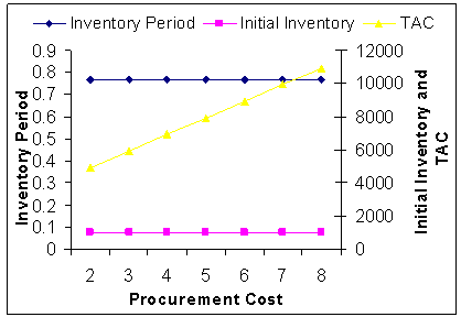Figure 7. Procurement Cost (Cp) Vs. Optimal Total Average Cost (TAC*)

In Table and Figure 7, we find that as the Procurement Cost increases, the optimal total average cost also increases. Further, an increase of 20% in procurement cost creates about % increase in optimal total average cost. Thus there exists a positive correlation between procurement cost and optimal total average cost.

Table 5. Holding Cost       Vs. Optimal Total Average Cost (TAC*)       Holding Cost (CH) % Change Inventory Period (t1*) Initial Inventory Level (S) Optimal Total Average Cost (TAC*) 25 -50 0.852457 1000.151914 7076.74 30 -40 0.806937 1000.127804 7000.06 40 -20 0.729722 1000.092711 6878.45 50 0 0.666704 1000.069063 6796.76 60 20 0.614296 1000.052516 6748.27 70 40 0.570028 1000.040569 6726.13 80 60 0.532140 1000.031717 6724.59

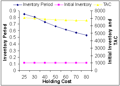Figure 8. Holding Cost Vs. Optimal Total Average Cost (TAC*)

In Table and Figure 8, we find that as holding cost increases, the optimal inventory period, optimal initial inventory level as well as optimal total average cost decreases. Moreover, about 20% increase in holding cost causes about 7.86%, 0.002% and 0.71% decrease in optimal inventory period, optimal initial inventory level and optimal total average cost respectively, which indicates that holding cost has negative correlation with optimal inventory period, optimal initial inventory level and optimal total average cost.

Table 6. Deterioration Cost (CD) Vs. Optimal Total Average Cost (TAC*)       Deterioration Cost (CD) % Change Inventory Period (t1*) Initial Inventory Level (S) Optimal Total Average Cost (TAC*) 40 -60 0.763809 1000.107336 6871.06 60 -40 0.764636 1000.107707 6892.15 80 -20 0.765457 1000.108077 6913.11 100 0 0.766271 1000.108444 6933.95 120 20 0.767079 1000.108810 6954.66 140 40 0.767881 1000.109173 6975.25 160 60 0.768676 1000.109534 6995.73

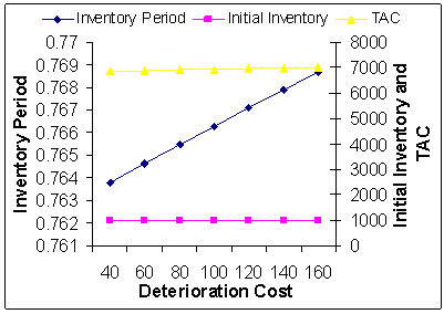Figure 9. Deterioration Cost (CD) Vs. Optimal Total Average Cost (TAC*)

In Table and Figure 9, we observe that as the deterioration cost increases, the optimal inventory period, optimal initial inventory level and optimal total average cost also increase. Numerically, an increase of 20% in deterioration cost amounts to about 0.11%, 0.0001% and 0.30% increase in optimal inventory period, optimal initial inventory level and optimal total average cost respectively. Here deterioration cost shows a positive correlation with optimal inventory period, optimal initial inventory level and optimal total average cost.

Table 7. Shortage Cost (Cs) Vs. Optimal Total Average Cost (TAC*)       Shortage Cost (Cs) % Change Inventory Period (t1*) Initial Inventory Level (S) Optimal Total Average Cost (TAC*) 56 -30 0.672614 1000.071102 6149.32 64 -20 0.707900 1000.084037 6400.12 72 -10 0.738871 1000.096506 6662.44 80 0 0.766271 1000.108444 6933.95 88 10 0.790685 1000.119826 7212.81 96 20 0.812576 1000.130648 7497.59 104 30 0.832315 1000.140919 7787.12

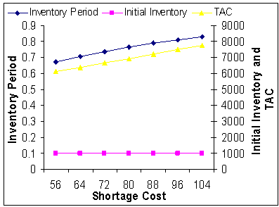Figure 10. Shortage Cost (Cs) Vs. Optimal Total Average Cost (TAC*)

In Table and Figure 10, we find that as the shortage cost increases, the optimal inventory period, optimal initial inventory level and optimal total average cost also increase. More exactly, an increase of 30% in shortage cost amounts to about 8.62%, 0.003% and 12.30% increase in optimal inventory period, optimal initial inventory level and optimal total average cost respectively. Here shortage cost shows a positive correlation with optimal inventory period, optimal initial inventory level and optimal total average cost.

Table 8. Lost Sales Cost (CL) Vs. Optimal Total Average Cost (TAC*)       Lost Sales Cost (CL) % Change Inventory Period (t1*) Initial Inventory Level (S) Optimal Total Average Cost (TAC*) 10 -50 0.762606 1000.106797 6921.18 12 -40 0.763348 1000.107129 6923.75 16 -20 0.764818 1000.107790 6928.87 20 0 0.766271 1000.108444 6933.95 24 20 0.767706 1000.109093 6938.99 28 40 0.769123 1000.109737 6943.99 30 50 0.769825 1000.110057 6946.47

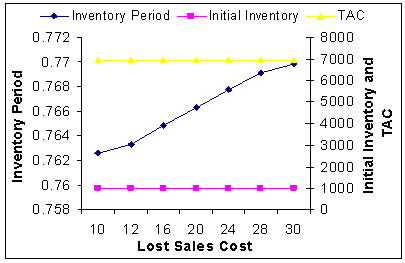Figure 11. Lost Sales Cost (CL) Vs. Optimal Total Average Cost (TAC*)

In Table and Figure 11, we find that as lost sales cost increases, the optimal inventory period, optimal initial inventory level as well as optimal total average cost also increases. Moreover, about 40% increase in lost sales cost causes about 0.37%, 0.0001% and 0.15% increase in optimal inventory period, optimal initial inventory level and optimal total average cost respectively, which indicates that lost sales cost has a positive correlation with optimal inventory period, optimal initial inventory level and optimal total average cost.

Table 9. Cycle Time       Vs. Optimal Total Average Cost (TAC*)       Cycle Time(T) % Change Inventory Period (t1*) Initial Inventory Level (S) Optimal Total Average Cost (TAC*) 0.5 -50 0.384319 1000.007632 10823.61 0.6 -40 0.458336 1000.017765 9319.84 0.7 -30 0.533458 1000.032003 8322.55 0.8 -20 0.609763 1000.051209 7651.19 0.9 -10 0.687336 1000.076338 7207.34 1.0 0 0.766271 1000.108444 6933.95 1.1 10 0.846672 1000.148702 6796.85

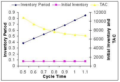Figure 12. Cycle Time Vs. Optimal Total Average Cost (TAC*)

In Table and Figure 12, we see that as cycle time increases, the optimal inventory period and optimal initial inventory level show an increasing trend whereas optimal total average cost shows a diminishing trend. In fact, about 10% increase in cycle time amounts to approx. 10.49% and 0.004% increase in optimal inventory period and optimal initial inventory level respectively but 1.98% decrease in optimal total average cost. Thus, cycle time is positively correlated with optimal inventory period and optimal initial inventory level whereas it is negatively correlated with optimal total average cost.

Table 10. Demand Parameter (n) Vs. Optimal Total Average Cost (TAC*)       Demand Parameter (n) % Change Inventory Period (t1*) Initial Inventory Level (S) Optimal Total Average Cost (TAC*) 2 50 0.766271 1000.201396 8270.73 3 -25 0.766271 1000.140977 7441.61 4 0 0.766271 1000.108444 6933.95 5 25 0.766271 1000.088111 6591.56 6 50 0.766271 1000.074199 6345.14 7 75 0.766271 1000.064081 6159.36 8 100 0.766271 1000.056391 6014.29

In Table and Figure 13, we see that as demand parameter increases, the optimal inventory period remains unaffected whereas optimal initial inventory level as well as optimal total average cost show diminishing trend. Further, an increase of 50% in demand parameter creates about 0.003% and 8.49% decrease in optimal initial inventory level and optimal total average cost respectively, which indicates that demand parameter is negatively correlated with optimal initial inventory level and optimal total average cost.

Figure 13. Demand Parameter (n) Vs. Optimal Total Average Cost (TAC*)

Table 11. Average Arrival Rate(λ) Vs. Optimal Total Average Cost (TAC*)       Average Arrival Rate(λ) % Change Inventory Period (t1*) Initial Inventory Level (S) Optimal Total Average Cost (TAC*) 19 -13.62 0.766271 1000.108444 6863.95 20 -9.08 0.766271 1000.108444 6908.95 21 -4.54 0.766271 1000.108444 6923.95 22 0.00 0.766271 1000.108444 6933.95 23 4.54 0.766271 1000.108444 6938.95 25 13.62 0.766271 1000.108444 6943.95 28 27.24 0.766271 1000.108444 6948.95

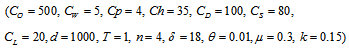
Figure 14. Average Arrival Rate(λ) Vs. Optimal Total Average Cost (TAC*)

In Table and Figure 14, we observe that as average arrival rate increases, the optimal total average cost also increases. In fact, about 27.24% increase in average arrival rate amounts to approx. 0.22% increase in optimal total average cost. Moreover, average arrival rate shows a positive correlation with optimal total average cost.

Table 12. Average Service Rate (δ) Vs. Optimal Total Average Cost (TAC*)       Average Service Rate (δ) % Change Inventory Period (t1*) Initial Inventory Level (S) Optimal Total Average Cost (TAC*) 18 -14.29 0.766271 1000.108444 6943.95 19 -9.52 0.766271 1000.108444 6938.95 20 -4.76 0.766271 1000.108444 6933.95 21 0.00 0.766271 1000.108444 6928.95 22 4.76 0.766271 1000.108444 6918.95 23 9.52 0.766271 1000.108444 6898.95 24 14.29 0.766271 1000.108444 6833.95

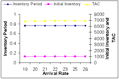
Figure 15. Average Service Rate (δ) Vs. Optimal Total Average Cost (TAC*)

In Table and Figure 15, we find that as average service rate increases, the optimal total average cost decreases. Numerically, about 14.29% increase in average service rate amounts to approx. 1.37% decrease in optimal total average cost. Moreover, average service rate shows a negative correlation with optimal total average cost.

Table 13. Deterioration Coefficient (θ)Vs. Optimal Total Average Cost (TAC*)             Deterioration Coefficient(θ) % Change Inventory Period (t1*) Initial Inventory Level (S) Optimal Total Average Cost (TAC*) 0.005 -50 0.760886 1000.053014 6614.41 0.006 -40 0.761977 1000.063909 6677.72 0.008 -20 0.764138 1000.085987 6805.24 0.010 0 0.766271 1000.108444 6933.95 0.012 20 0.768376 1000.131277 7063.85 0.014 40 0.770455 1000.154482 7194.94 0.015 50 0.771484 1000.166222 7260.93

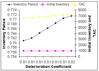Figure 16. Deterioration Coefficient (θ)Vs. Optimal Total Average Cost (TAC*)

In Table and Figure 16, we observe that as deterioration coefficient increases, the optimal inventory period, optimal initial inventory level and optimal total average cost also increases. Actually, about 40% increase in deterioration coefficient causes about 0.55%, 0.005% and 3.76% increase in optimal inventory period, optimal initial inventory level and optimal total average cost respectively, which indicates that deterioration coefficient has positive correlation with optimal inventory period, optimal initial inventory level and optimal total average cost.

Table 14. Life Time (μ) Vs. Optimal Total Average Cost (TAC*)       Life Time (μ) % Change Inventory Period (t1*) Initial Inventory Level (S) Optimal Total Average Cost (TAC*) 0.1 -67 0.765828 1000.114911 6924.45 0.2 -33 0.765991 1000.113190 6928.00 0.3 0 0.766271 1000.108444 6933.95 0.4 33 0.766676 1000.099140 6942.32 0.5 67 0.767212 1000.083742 6953.17 0.6 100 0.767887 1000.060714 6966.54 0.7 133 0.768709 1000.028523 6982.51

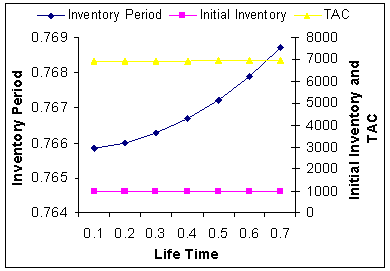Figure 17. Life Time (μ) Vs. Optimal Total Average Cost (TAC*)

In Table and Figure 17, we observe that as life time of deteriorating items increases, the optimal inventory period and optimal total average cost increases whereas optimal initial inventory level diminishes. Numerically, about 67% increase in life time causes about 0.12% and 0.28% increase in optimal inventory period and optimal total average cost respectively but 0.003% decrease in optimal initial inventory level. Thus life time is positively correlated with optimal inventory period and optimal total average cost but it is negatively correlated with optimal initial inventory level.

Table 15. Backlogging Coefficient (k)Vs. Optimal Total Average Cost (TAC*)             Backlogging Coefficient(k) % Change Inventory Period (t1*) Initial Inventory Level (S) Optimal Total Average Cost (TAC*) 0.06 -60 0.727506 1000.091806 5742.59 0.09 -40 0.739399 1000.096728 6125.36 0.12 -20 0.752279 1000.102239 6521.71 0.15 0 0.766271 1000.108444 6933.95 0.18 20 0.781528 1000.115473 7364.90 0.21 40 0.798229 1000.123489 7818.08 0.24 60 0.816589 1000.132696 8297.89

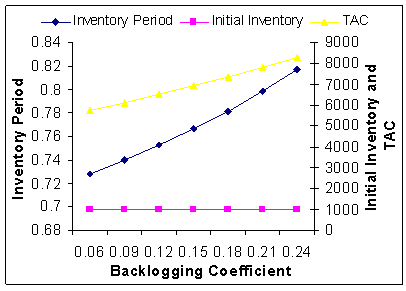Figure 18. Backlogging Coefficient (k)Vs. Optimal Total Average Cost (TAC*)

In Table and Figure 18, we find that as the backlogging coefficient increases, the optimal inventory period, optimal initial inventory level and optimal total average cost also increase. More exactly, an increase of 40% in backlogging coefficient amounts to about 4.17%, 0.002% and 12.75% increase in optimal inventory period, optimal initial inventory level and optimal total average cost respectively. Here backlogging coefficient shows a positive correlation with optimal inventory period, optimal initial inventory level and optimal total average cost.

5. Conclusions

In the present paper, we have developed an inventory model for perishable items with power form time dependent demand and quadratic deterioration rate. This type of demand if occurs, then managers develop a different policy other than the conventional policy based on general ramp pattern. In cases where large portion of demand occurs at the beginning of the period we use n > 1 and if it occurs at the end of the period, we use 0 < n < 1. Constant demand rate corresponds to n = 1 and n = ∞ corresponds to instantaneous demand. Shortages are allowed and the backlogging rate is dependent on the duration of waiting time for the next replenishment and varies inversely. Shortages are partially backlogged in this model. Behaviours of different parameters have been discussed through the numerical example and sensitivity analysis. A future study will incorporate more realistic assumptions in the proposed model such as stochastic nature of demand and deterioration.

ACKNOWLEDGEMENTS

The authors are highly thankful to the referees and editors for improving the paper in the present form and NBHM Grant 2/48(6) 2012/NBHM/R&DII/13614.