-
Paper Information
- Paper Submission
-
Journal Information
- About This Journal
- Editorial Board
- Current Issue
- Archive
- Author Guidelines
- Contact Us
American Journal of Operational Research
p-ISSN: 2324-6537 e-ISSN: 2324-6545
2012; 2(6): 104-119
doi:10.5923/j.ajor.20120206.04
Profitable Vehicle Routing Problem with Multiple Trips: Modeling and Variable Neighborhood Descent Algorithm
 Abstract
 Reference
 Full-Text PDF
 Full-text HTML
Ahlem Chbichib1, Racem Mellouli2, Habib Chabchoub3
1Department of Quantitative Methods, Faculty of Economic Sciences and Management, Sfax, 3018, Tunisia
2Department of computer and quantitative methods, the Higher School of Management, Sfax, 3018, Tunisia
3Department of Quantitative Methods, Institute of the High Commercial Studies, Sfax, 3018, Tunisia
Correspondence to: Ahlem Chbichib, Department of Quantitative Methods, Faculty of Economic Sciences and Management, Sfax, 3018, Tunisia.
| Email: |  |
Copyright © 2012 Scientific & Academic Publishing. All Rights Reserved.
In this paper, we tackle a new variant of the Vehicle Routing Problem (VRP) which combines two known variants namely the Profitable VRP and the VRP with Multiple Trips. The resulting problem may be called the Profitable Vehicle Routing Problem with Multiple Trips. The main purpose is to cover and solve a more complex realistic situation of the distribution transportation. The profitability concept arises when only a subset of customers can be served due to the lack of means or for insufficiency of the offer. In this case, each customer is associated to an economical profit which will be integrated to the objective function. The latter contains at hand the total collected profit minus the transportation costs. Each vehicle is allowed to perform several routes under a strict workday duration limit. This problem has a very practical interest especially for daily distribution schedules with limited vehicle fleets and short course transportation networks. We point out a new discursive approach for profits quantification which is more significant than those existing in the literature. We propose four equivalent mathematical formulations for the problem which are tested and compared using CPLEX solver on small-size instances. Optimal solutions are identified. For large-size instance, two constructive heuristics are proposed and enhanced using Hill Climbing and Variable Neighborhood Descent algorithm based on a specific three-arrays-based coding structure. Finally, extensive computational experiments are performed including randomly generated instances and an extended and adapted benchmark from literature showing very satisfactory results.
Keywords: Profitable Vehicle Routing Problem, Multiple Trips, Mixed Integer Linear Programming, Constructive Heuristics, Hill Climbing, Variable Neighborhood Descent
Cite this paper: Ahlem Chbichib, Racem Mellouli, Habib Chabchoub, Profitable Vehicle Routing Problem with Multiple Trips: Modeling and Variable Neighborhood Descent Algorithm, American Journal of Operational Research, Vol. 2 No. 6, 2012, pp. 104-119. doi: 10.5923/j.ajor.20120206.04.
Article Outline
1. Introduction
- Nowadays, effective management of the supply chain is recognized as a determinant key of competitiveness and success for manufacturing and distribution organizations. The problems of routing goods from depots to consumers or between different logistical sites are very important. Drawing adequate plans may produce significant savings for many distribution systems. Therefore, the Vehicle Routing Problem (VRP) is a well-known problem studied in Operational Research. It deals with finding the optimal delivery routes configuration from one or several depots to a number of customers using a fleet of capacitated vehicles, while satisfying some constraints. The solution of a VRP is a set of minimum cost routes which fulfill the customers’ requirements. In the classical version of the problem, only one depot is considered with an unlimited fleet of vehicles where each vehicle performs exactly one circuit. Several operational constraints can be considered in more practical applications of the VRP.In this research, we focus on two variants of the VRP: the Profitable VRP and the VRP with Multiple Trips, which we combine to obtain a new variant not addressed in the literature to our knowledge and involving a new challenge in term of solving approaches. This problem which can be named the Profitable Vehicle Routing Problem with Multiple Trips (PVRPMT) calls for the determination of a set of routes for a given heterogeneous set of vehicles visiting a selective subset of customers such that: i) it is difficult, if not impossible, to visit all customers for a lack of logistical means or for insufficiency of the offer; ii) each visited customer provides a fixed profit that is recognized in the objective function to maximize. The latter is the difference between the total profit generated by the all visits and the resulting total transportation cost; iii) each vehicle may perform several routes in the same planning period but does not exceed a strict duration limit (temporal capacity); iv) for each route, the total load does not exceed the vehicle capacity (physical capacity). The motivation to study this problem come not only from its theoretical interest but also from its practical relevance. For example, the size of the vehicle fleet indicates the capital invested in logistics resources. That the reduction of this size is naturally more desirable, the problem counts as a strategic choice in the problem reading to guide the optimization towards reducing both capital and operating (scheduling) costs. In this situation, there might be a trade-off between higher scheduling costs and lower vehicle ownership-based costs (and eventually associated driver salaries-based costs). Otherwise, this problem is very practical where daily drivers’ schedules must be achieved with a limited vehicle fleet and short-distance distribution networks. Furthermore, when we are unable to respond to all costumer requests, the problem reading should be different. A subtle selection of costumers to be served is required. It should be based on a clear and measurable criterion. It is therefore important to define a significantly manner to classify customers according to their importance, behavior and costs implications, and to translate this into a global criterion that can be optimized as the total cost associated with the transportation program. This issue of profitability will be raised when the instances are to be conceived and tested, because most companies do not have a carefully designed evaluation of each costumer’s profit. The latter should not only be related to the volume of its current request but must take into account other considerations, related to the future potentials of this costumer. And the value must also be reasonably projected on a coherent scale with the transportation costs that appear in the objective function in order to ensure significant aggregation-based assessments for the computed solutions.The addressed problem concerns the PVRPMT as a new variant of practical VRP. Note that this kind of problems would be attractive in particular for planning mechanisms of ERP software which must integrate a miscellaneous range of situations of management and control. For a more devoted emphasis mainly to the operational context, our objective is multiple with this problem combining at hand: the maximization of the total collected profit, the minimization of the total routing costs and indirectly the maximization of the use of resources (vehicles and drivers). The issue of different mathematical models for this problem is to be addressed and used to seek solution optimality for small-size instances. Giving the complexity of the problem which is NP-hard, two constructive polynomial heuristics with two different greedy-based constructions will be proposed as a first approach to solve the large-size instances. Their effectiveness is tested and then enhanced, in a second solving approach, with an iterative ameliorative procedure using successive local searches with multiple and sequential neighborhood structures. For instances generation, we point out a new and quick discursive approach for profits quantification which is more significant than those existing in the literature.The remainder of this paper is organized as follows. Section 2 reviews the related research literature. In section 3, we formally present the optimization problem PVRPMT with a detailed theoretical graph description and we introduce the corresponding proprieties and notations. Furthermore, we determine this problem complexity. In Section 4, based on two strategies of sub-tours elimination constraints, we provide four mathematical models of the problem including MILP and 0-1 ILP. Section 5 describes two constructive heuristics and an enhancement procedure based on the Variable neighborhood Descent algorithm (VND). The computational experiment is presented in Section 6 to obtain insights about the different performances of the optimizing proposed algorithms. This section begins with a new precision about the evaluation of profitability indices to be incorporated into the numerical instances’ files and subsequently into the computation of the objective functions in adequacy with the measures adopted for the transportation costs. We draw conclusions and discuss future research directions in Section 7.
2. Literature Review
- The problem we focus on is a combination of the two known variants such that: the vehicle routing problem with multiple trips or with multiple uses of vehicles (noted by VRPMT or VRPM) and the profitable vehicle routing problem (PVRP). To the best of our knowledge, these problems are studied separately in literature, excepting some special recent works[2, 3, 5], but with time windows considerations. For the latters, the concept of Multiple Trips is obtained indirectly by imposing a duration limit on each tour and not on the workday duration. Thus, the problem may look like a Capacitated VRP, where the multiple uses of vehicle is a consequence since the tours duration limit is fixed sufficiently small. So, the tours could be seen as parallel tours conducted by several vehicles. However, the integration of time windows constraint into the same problem gives the importance to the tours’ order and consequently gives a special (restricted) Multiple Trips consideration. In this section, we devote two sub-sections to review the literature of the VRPMT and the PVRP.
2.1. The Vehicle Routing Problem with Multiple Trips
- The VRPMT is an extension of the classical VRP in which the same vehicle may perform several routes in the same planning period (workday). In this case, the fleet includes a fixed number of available vehicles. However, the duration of a vehicle workday which is made of a set of successive routes does not exceed a certain limit.This problem has a very practical importance. For example, in the home delivery of perishable goods like food, routes are of short duration and must be combined to form a complete workday[1]. Some real-world cases dealing with this kind of problem appear in applicative research publications. For instances, note the paper of Brandao et al. 1997[6] which studies the VRP in Burton’s Biscuit Ltd; and the case study of the logistical activities of Santa Fe Indonesia (precisely in the office of Jakarta, a company specialized on relocation services to individuals as well as companies) which is considered in[7]. Derigs et al. 2011[8] study some real cases dealing with this problem from a consultancy company in the air cargo transportation field (air cargo road feeder services). Planned and ad-hoc tasks, different resources and environment constraints are taken into account, such as driving time with breaks, working time with minimum requirements in relation to the health and the safety of persons performing mobile road transport activities. These problems deals with different applications, such as: the transportation of live animals to a slaughterhouse, the transportation of the meals or the flight food from a central kitchen to the aircraft, the transportation of goods from suppliers to retailers using one or more cross-docks. More additional constraints, such as time windows, split delivery, heterogeneous fleet, are considered respectively in[9, 10, 11and 12]. Grünert et al. 1999[13] develop a decision support system (DSS) which is designed in order to assist planners of the German postal service at the Deutsche Post AG. The main goal is to reduce the costs of the letter-mail transportation. In[14], a vehicle routing problem including multiple trips in a health care organization which operates about 240 buildings of medical offices in Southern California is treated. Finally, we mention Hernandez et al. 2009[15] which present a VRPMT applied in a context of optimizing the agronomic performance and its impact on the environment. In the academic literature, the papers treating the VRPMT consider in general additional constraints mainly the time windows. Azi et al. 2007[1] study this problem with time windows consideration and a single vehicle’s use. The extension for multi-vehicle version is tackled by Azi et al.[2, 3, 4] and Macedo et al. 2011[5]. Other works include also both multiple trips and time windows such as[6, 7, 8, 11, 12, 14, 15, 16, 17, 18, 19 and 20]. The overtime constraint is incorporated to the VRPMT in[14, 16, 21, 22, 23 and 24]. Heterogeneous fleet is considered with this problem in[7, 10, 12, 16 and 27]. Some VRPMT are studied by including a products compatibility constraint which forbidden to gather in a same vehicle route two or more different categories of goods[7, 8, 16, 24, and 27]. The multiple trips constraint is used in VRP with backhaul in[7 and 12], combined with allowed split delivery case in[12], with location problem in[25 and 26], with a planning horizon of several days in[14 and 27], with multiple depots in[28], with meal breaks during the driving time in[11]. The problem is studied in a dynamic environment in[4 and 8]. In term of solving methods, few papers develop exact approaches for the VRPMT, because of the problem’s complexity, such as[1, 2, 5, 15 and 17] using MILPs, column generation with branch-and-price algorithm and network flow-based models. Note that solving the VRPMT may consist on solving a routing and packing problem. In this level, different heuristics and metaheuristics are developed. For the routing phase, we can distinguish some constructive heuristics used to obtain an initial solution, such insertion heuristics used in[3, 4, 10, 14, 20, 22, 27 and 29], the Clark and Wight algorithm[24, 25 and 31], the modified Clark and Wight algorithm[25 and 31], the nearest neighborhood method[25 and 29], clustering algorithms[7, 19 and 24], the sweep-based algorithm[20, 21, 28 and 32], set covering-based approaches[7 and 32] and the petal method[32]. The initial obtained solutions are enhanced by different methods: we find the tabu search in[6, 13, 14, 18, 19, 20, 21, 23, 25, 27, 28 and 29], the simulated annealing in[3, 25, 26 and 31], neighborhood search based on insertion moves in[10, 18, 22, 24, 25, 29 and 31], on swap moves in[22, 24, 25, 26, 29 and 31], on 2-opt in[18 and 25], on adaptive memory in[21 and 30]. Other specific neighborhood search algorithms are proposed such as large neighborhood search in[3 and 4], guided neighborhood search in[8]. In[8], we find also a decomposition approach. In[18], a filter and fan procedure is developed. For the packing phase, some well-known heuristics for bin packing problems are used, specially the best fit decreasing in[16, 22, 24, 25 and 30]. In[8], a greedy packing procedure is used and a fuzzy theory-based method is proposed in[33].The VRP with multiple trips, but no other additional constraints, is addressed through heuristics in Brandao and Mercier 1998[7], Taillard et al. 1996[23], Olivera and Viera 2007[21], Petch and Salhi 2004[22].
2.2. The Vehicle Routing Problem with Profit
- VRP with profits are a generalization of the vehicle routing problems. Given a fixed-size fleet of vehicles, it might not be possible to serve all customers. Thus, a known profit is associated with each demand node and the customers must be chosen based on their associated profit minus the travelling cost to reach them in the solution. The idea to associate a known profit at each customer is made by Dell’Amico et al. 1995[35]. The constraint to visit all the customers is relaxed, but for each unvisited customer a given penalty has to be paid. The objective function is to find a balance between these penalties and the cost of the tour. Profits are explicitly considered both in the Vehicle Routing Problem (PVRP) and the Traveling Salesman Problem with Profits (TSPP), as stated by Feillet et al. 2005[34] in an excellent comprehensive survey. The TSPP can be formulated as a discrete bi-criteria optimization problem where the two goals are referred: maximizing the profit and minimizing the traveling cost. It is also possible to use one of the goals as the objective function and the other as a constraint. These problems can be divided into three categories according to Feillet et al. 2005[34]: a) the Profit Tour Problem (PTP), b) the Selective TSP (STSP), and c) the Prize–Collecting TSP (PCTSP). For the first problem (PTP), the objective is to maximize the difference between the total collected profit and the traveling cost. Feillet et al. 2005[34] survey lists various modeling approaches to TSPP and exact methods as well as heuristic solution methods. Archetti et al. 2009[36] study the capacitated version of the PTP and propose exact and heuristic procedures for it. More recently, the authors[37] develop an exact approach based on a branch-and-price algorithm. A restricted master heuristic is applied at each node of the branch-and-bound tree in order to obtain primal bound values. For the second problem which is known through three equivalent names in the literature: the Orienteering Problem (OP), the Selective TSP (STSP), or the Maximum Collection Problem (MCP), the objective is to maximize the collected profit such that the total traveling cost or distance does not exceed a certain upper bound. The multi-vehicles version of the OP is very similar to the VRP, except that vehicles are assumed to be with unlimited capacity and there is a time constraint on each tour. This problem is called the Team Orienteering Problem (TOP). Recently, Vansteenwegen et al. 2011[43] provides a survey of the existing OP and TOP. In this paper, the applications and the solving approaches about the two problems is reviewed listing various modeling approaches and exact as well as heuristic solution methods. In addition, many relevant variants of these problems are formally presented. For the third problem which is named the Prize– Collecting TSP or also known as the Quota TSP concerns the determination of a tour with the minimum total traveling cost where the collected profit or prize is greater than a lower bound.Note that the PVRP is also a kind of PTP when considering comparing to TSPP that vehicles have physical loading capacities. In[38], The PVRP is applied in the reverse logistics where a firm aims to collect cores from its dealers. The problem is an extension of the classical multi-depots vehicle routing problem (MDVRP) in which each visit to a dealer is associated with a gross profit and an acquisition price to be paid to take the cores back. First, two mixed-integer linear programming (MILP) are presented. Then, a Tabu Search-based heuristic is proposed to solve medium and large-sized instances. In[39], the research deals with a VRP in which the total profit is to be maximized subject to market competition. The PTP in a dynamic environment is considered in[40]. In this problem, the rewards (profits) are unknown for the customers which are not yet served. Indeed, the rewards depend on competitors’ prices and auctions. In another extension of the problem, the profit is associated to each edge non to vertices. The problem is then called the Profitable Arc Routing Problem (PARP). Archetti et al. 2010[41] study the capacitated undirected version (UCARPP) and develop a branch-and- price algorithm, several heuristics based on Variable Neighborhood Search (VNS) and two Tabu Search heuristics. Zachariadis et al. 2011[42] propose another local search approach for the UCARPP. Two solution neighborhoods are considered and the overall search is coordinated by the use of the promises concept.The problem studied in this paper is a new extension which combines the two previous variants.
3. Problem Definition and Notation
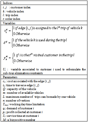
3.1. Problem Description and Notation
- We consider a complete undirected graph G = (V, E), where V= {0… n} is a set of vertices and E is a set of edges. Vertex 0 represents the depot and a fleet of vehicles k = {1… m} is based. Each vehicle has a limited capacity Q (or Qk if with heterogeneous fleet) and a maximum number of trips L. Note that, the parameter L is defined to facilitate the problem formulation and can be used as a real constraint, i.e. as a limit to be respected. However, the best value of L can be experimentally identified. An edge (i,j)∈E represents the possibility to travel from customer i to customer j. A non-negative demand qi, profit pi, and time service Si, are associated with each customer i (with setting p0=q0=0). A travel time tij and cost cij are associated with each edge (i,j)∈E. Each vehicle starts and ends its tour at vertex 0, and can visit any subset of customers with a total demand that does not exceed the used vehicle capacity Q. In addition, there exists a time horizon denoted by the duration limit Tmax which establishes the duration of a workday. It is assumed that all parameters are nonnegative integers and the environment is deterministic. This problem named the PVRPMT consists on determining a set of routes and to assign each route to one vehicle, such that the same vehicle can be used by several routes while respecting the time horizon capacity. The objective is to maximize the difference between the total collected profit and the cost of the total traveled distance. Note that the following properties:• The optimal solution may be composed by a subset of customers.• Each route starts and ends at the depot,• The total customers’ demand in the same route does not exceed the physical capacity of used vehicle,• The duration of routes assigned to the same vehicle does not exceed Tmax.• The profit associated at each customer is fixed and can be collected by any vehicle.
3.2. Problem Complexity
- Olivera and Viera[21] proved that the VRPMT is NP-hard as well as the PVRP[34]. The studied problem represents the combination of these two NP-hard problems. This makes it also NP-hard. In addition, PVRPMT is a generalization of the classical VRP. There are instances of PVRPMT in which there exist enough vehicles in the fleet able to optimally visit during the workday all customers using one vehicle for each tour. These cases are naturally reduced to a classical VRP. As the VRP is an NP-hard[22], the PVRPMT is also NP-hard.
4. Mathematical Models for the PVRPMT
- The design of the VRP solution stands against the presence of the sub-tours. For that, different sub-tours elimination constraints are proposed. The most classical constraint and the most used in the literature can be written in this way:
 | (1) |
|
4.1. Modeling with 0-1 Integer Linear Programming
- We start with the idea to specify for each assigned customer his order in the trip. This idea has been applied in the scheduling problem. For each job, we determine the position of the job in the sequence. We use the visit order of customer i in the trip in order to eliminate the invalid tours. Accordingly, we eliminate the subset S and the associated constraints. We consider the following binary decision variables:

 A new decision variable
  is added and informs about the visit order of customer i in the trip l. Based on the choice of the principal variable in the formulation, we can distinguish two different mathematical models.• First formulation: 0-1ILP1 with
  as principal variables. Here, the second variable
  is used just to make the connection between the edge and the vertices. The resulting formulation is the following:
 | (2) |
 | (3) |
 | (4) |
 | (5) |
 | (6) |
 | (7) |
 | (8) |
 | (9) |
 | (10) |
 | (11) |
 | (12) |
 | (13) |
 | (14) |
 as principal variables In this model, we conserve the constraints which establish the relation between
  and
and  such in ILP1. When it is possible, we integrate the variable
 in the objective function and in the constraints. The objective is to test the influence of this transformation on the upper bound and to know which expression can conserve much more information if the integrity constraints are relaxed. The resulting model is as follow:
  | (15) |
 | (16) |
 | (17) |
 | (18) |
 | (19) |
 | (20) |
 | (21) |
 | (22) |
 | (23) |
 | (24) |
 | (25) |
 | (26) |
 | (27) |
4.2. Modeling with Mixed Integer Linear Programming
- To overcome the limitation of the classical sub-tours elimination constraint, Miller et al. 1960[44] propose a new ones which are corrected by Kara et al. 2004[45]. In this level, we propose an adaptation of these constraints to our problem. For that, we remove the decision variable
 and we define Ui. as an associated variable to customer i used to reformulate the sub-tour elimination constraints;Firstly, we present the ordinary model. Then an extension of this model with some proposed cuts.• Third formulation: MILP1 (without cuts)The formulation is the following:
  | (28) |
 | (29) |
 | (30) |
 | (31) |
 | (32) |
 | (33) |
 | (34) |
 | (35) |
 which informs about the used vehicle. So, the correspondent constraints which establish the relation between the two decision variables will be adjoined.
  The formulation becomes:
 | (36) |
 | (37) |
 | (38) |
 | (39) |
 | (40) |
 | (41) |
 | (42) |
 | (43) |
 | (44) |
 | (45) |
 | (46) |
 | (47) |
4.3. The Heterogeneous Fleet Case
- In this subsection, we proposed a formulation extension to solve the special case of PVRPMT with heterogeneous fleet. So, each vehicle k has its own capacity
 . Then, some modifications on MILP2 are done. The constraint (4.3) is replaced by (5.3). The constraints (4.6) and (4.7) are replaced respectively by (5.6) and (5.7):
 | (48) |
 | (49) |
 | (50) |
5. Solving Algorithms
- The present section is devoted to the description of the main steps of the implemented algorithms. We start by explaining the solution coding scheme. Then, constructive heuristics used to build initial feasible solutions to the problem are described. Finally, improvement procedures based on Hill Climbing and Variable Neighborhood Descent (VND) are proposed.
5.1. Solution Coding Scheme
- To further speed up the computation, we use tree-array data structure to represent a solution. The information concerning the customer is stored into the first array (V1[j]). So, its size is equal to the number of customers n (we eliminate the deposit from the solution representation). First, the visited customers are stored adjacently in the order of visit. Then, the unvisited customers are inserted in the end of the array. It is important to know the start and the end of each trip. This information is done by the second array (V2[j]). This latter is a binary vector. Finally, the third array (V3[j]) informs about the index of the used vehicle to visit the correspondent customer. Using this structure, the lecture of the solution is clear and easy, and changes can be performed very quickly and in a constant time. The solution is coded as follows:Let the matrix V[i][j] with i
 {1, 2, 3}and j
  {1, 2,…n} be the following:
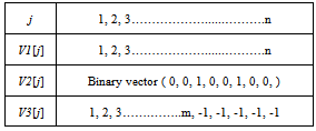
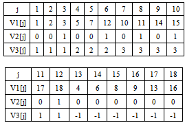
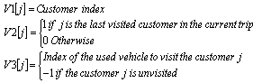 Figure 1 represents an illustrative example with 5 short routes, 18 customers and 3 vehicles and table 4 represents the relative solution code.
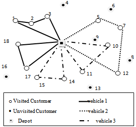 | Figure 1. Illustrative Example |
|
5.2. Constructive Heuristics for the PVRPMT
- The goal of this subsection is to construct good feasible solutions for the problem. We propose two greedy constructive heuristics. These heuristics use some local optimalities in certains steps of the algorithm.
5.2.1. Heuristic H1
- The insertion heuristic is used to build an initial feasible solution. In every iteration, the procedure evaluates all feasible insertions of unvisited nodes and selects the node representing the best insertion. An insertion is evaluated with the following criterion. Let i be some node in a tour and let j be a node candidate for the insertion. Let Chgact and Tmact denote the actual charge and the traveled time for the current used vehicle respectively. The insertion of j is feasible if the capacity constraint and the constraint of time duration are verified (i.e. (51) and (52) are verified):
 | (51) |
 | (52) |
 | (53) |
5.2.2. Heuristic H2
- This heuristic H2 is almost identical with heuristic H1 with the following basic difference : to construct the trip, we use the same previous procedure, but the used vehicle is not necessary kept in prior for the next trip. At each iteration, we choose the vehicle which has the longest remaining time service by breaking ties with the largest capacity order (see Figure 3).
 | Figure 2. Constructive Heuristic 1 |
 | Figure 3. Constructive Heuristic 2 |
5.3. Improvement Scheme
- For the PVRPMT, it is essential to have a neighborhood that changes the visit combinations for customers. Three kinds of moves including insertion move, swapping move and Cross exchange operator move are used to define a set of neighborhoods that allow the exploration of increasingly distant solutions from the incumbent to overcome local optimality and strive for global optimality. Our improvement phase consists on first developping three Hill Climbing algorithm (HCi, HCs, HCc) using the three neighborhood structures, then we test the influence of combining the three last algorithms in a Variable Neighborhood Descent procedure.
5.3.1. Hill Climbing Procedure
- The local search algorithms show its performance to solve various variants of routing problems. Here we use the Hill Climbing heuristic which belongs to the family of local search methods which often built on neighborhood moves that make small changes to the current solution. The insert move consists of removing one customer from a current position j (origin position) and putting him into another new position k. The destination route (i.e. the route that contains the new position) can be an existing route or a new one. To take into account all the possible moves, a new decision variable α is defined.
 All depends on the positions of j and k and the variable δ, we can distinguish different possible moves.* If j=k , three scenarios can be distingushed :• k is the position of the first visited customer in the current trip (i.e. V2[k-1]=1)- if α=prec the customer i will be inserted in the last trip (i.e. V2[k-1]=0,V2[k]=1 and V3[k]= V2[k-1])- if α=suiv no change in the initial solution• k is the last visited customer in the current trip (V2[k]=1)- if α=prec no change in the initial solution- if α=suiv the customer i will be inserted in the next trip (i.e. V2[k-1]=1,V2[k]=0 and V3[k]= V3[k+1]).• Otherwise : there is no change * If j≠k, according to the value of V2[k] two different cases can appear :• If, in the initial solution, (V2[k]=1) : two insert moves are presented- α=prec: i will be the last visited customer who belongs to the current trip (V2[i]=1 and (V3[i]= V3[k] ) .- α=suiv : i will be the first visited customer in the next trip (V2[i]=0 and (V3[i]= V3[k+1]).• if (V2[k]=0), the new solution will be presented as follows: V1[k] =V1[j], V2[k] =0 and V3[k] =V3[k-1].the swap move consists on exchanging two customers. In the new solution just the position of the two selected customers will be exchanged (V1[k] =V1[j]). The cross-exchange operator consists on interchanging non-consecutive customer segments between the same or two different routes with the restriction that the orientation of them be maintained.Remarq 3: Note that , to elliminate the neglected move, for the two first neighborhoods (insertion and swap), at least one from the two selected customers should represent a visited customer in the initail solution. For the cross-exchange operator, the two selected customers should be visited in the initail solution.
5.3.2. Variable Neighborhood Descent Algorithm
- The second idea is to test the influence of combining the three neighborhood structures in the same algorithm. So, we develop a variable neighborhood decent algorithm (VND).The VND is the simplest variant of the variable neighborhood search heuristic (VNS) which performs several descents with different neighborhoods until a local optimum for all considered neighborhoods is reached. Let
 denote a set of K neighborhood structures (i.e.,
  contains the solution that can be obtained by performing a local change on s according to the
  type).Step 1. Choose an initial solution s in S.Step 2. Set
  and
and  .Step 3. Perform a descent form s, using neighborhood
 . Let
. Let  be the resulting solution. If
  then set
 . Set
. Set . If
. If  then repeat Step 3.Step 4. If
  then go to Step 2; else stop.[46]
6. Computational Results
- In the following, obtained results concernening the performance of the different proposed mothods are reported. First, the test instances construction, the parameters choice and the profit quantification are presented. Then, the performance of the equivalent presented models are tested and compared. Finally, the last subsection is devoted to the heuristics procedures performance (contructive, Hill Climbing, VND). The MILPs and solving algorithms was tested on a Intel Core 2 Duo CPU 2.20 GHZ and 4.00 Go RAM. The codes are written in C++, using CPLEX librairies for the first part. All the algorithms were stopped before a computational time of one hour at atmost.
6.1. Test Instances and Parameters Choice
- The tests will be applied first on our own benchmark devoted for small-size instances and then on the benchmarks of Taillard et al. 1996[23] taken from the VRP library with adaptations and some extended data. In our benchmark, twenty small-size instances are generated randomly. A certain setting is used to obtain interesting instance values according to the practice and real-case situations. For each instance, we indicate the number of vertices n which ranges from 6 to 20. The customers are randomly distributed in two-dimension area, and the depot is set at point (0, 0). the fleet of vehicles m accounts for 2 or 3 vehicles. The vehicle physical capacity limit Q ranges from 1000 to 3000 kgs. The horizon time limit
 for all the small size instances is equal to 480 minutes (i.e. 8 hours of workday). Note that in the litterature according to[36], the profit
  of customer i depends on the three parameters namely: cons, h and the customer’s demand
  , where h is a random ratio number uniformly generated in the interval[0,1] and cons is a constant factor that measures the profit according to a sale turnover. In[36], the authers consider pi = (cons + h)qi and suppose that cons=0.5 indifferently with the level of greatness of the other values used for the instances data. This implies a lack of guarantee of a necessary coherence between the different values while the choices of the units and the level of greatness of the four used data are unambiguous: costomers’ demands qi , distances dij , transportation times tij and transportation costs cij.In our opinion, it is important to obtain meaningful and significant proportions of the profits according to the transportation costs. In our case, they are assimilated to dij . Concerning the profit calculation, we take as reference a general realistic model where the logistical cost represents between 5 and 10 per cent of the sale turnover, and the gross benefit may represent between 20 and 50 per cent of the sale turnover. So, it is possible to have a global profit which ranges almost between 3 and 5 times the gobal transportation cost. The distribution of this global profit on customers may respect the demand quantity qi of each customer i. Let qmax and qmin be respectively the greatest and the smallest value of all demand quantities. qmax and qmin can be associated respectively to αmax =5 and αmin =3 factors. We use a projetion to calculate the factor αi of the customer i according to his demand qi . In order to estimate the transportation cost, we calculate firstly the average distance, identify and αi and pi such as:
 | (54) |
 | (55) |
 | (56) |

6.2. Mathematical Models Experimentations
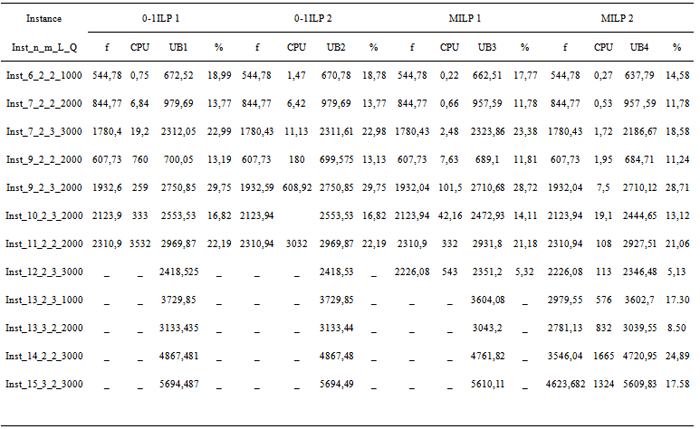
- In order to test the proposed models, we used the commercial solver CEPLEX 10.0. of ILOG ®. First, the four mathematical models are teted on the small size instances and the results are reported in Table 3.The optimal solution obtained by CPLEX is indicated under column f . The “_” means that we cannot obtain the optimal solution before the time limit. The column UB represents the solution of the linear relaxed problem (the upper bound). In addition, (%) represents the gap between the optimal solution and the relevant upper bound. (%) = (f-UB)/UB 100. We observe on Table 3 that the optimal value can be obtained within the time limit just for small size instances for the four mathematical models. For the instances where the number of vertices is superior to 17, the optimal solution cannot be determined. We can show also that computationnel time grow strongly with the increase of instance size. MILP 2 is able to solve more instances than the other proosed models and it clearly outperforms them in terms of computing time. In Table 4, we try to compare the performance of the four mathematical models by confronting the obtained upper bounds. We choose as reference the upper bound of the first mathematical model (UB1) and we calculate the deviation of the different upper bounds in comparison with the first. (%*)w =(UBw-UB1)/UB1 100 .Different remarks can be taken into account. First by comparing the two strategies, the 0-1 ILP and the MILP, it is very clear that the upper bounds obtained by the mixed integer programming are better than those obtained by the 0-1 integer programming for all the tested instances. For the 0-1ILP, the choice of the principal variable has not great influences on the upper bounds quality (for the majority of the tested instances the upper bound obtained by the two models are equal) but strongly affects the number of iterations. For the MILP, the upper bounds of the mathematical models with cuts are better than those without cuts. That shows the efficiency of these cuts. MILP2 is able to solve more instances than the other mathematical models and outperforms them in terms of computing time and the upper bound quality. So, we can judge that the additional constraints represent valid cuts for our model.
6.3. Heuristics Procedure Performance
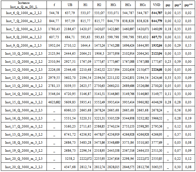
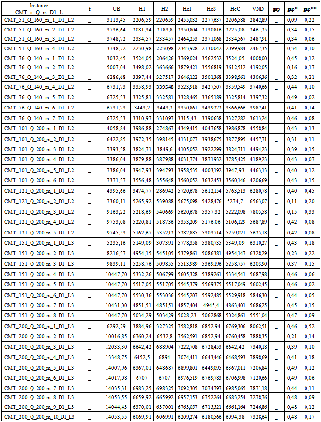
- To test and compare the performance of our heuristics, we compute the obtained gaps of the obtained solutions comparing to the linear upper bounds. These gaps are given: first for the two constructive heuristics bounds, second for the three Hill Climbing based solutions, and finally for enhancement by using the Variable Neighborhood Descent algorithm. Gaps are also computed comparing to the optimal solution for the small-size instances. Then, to know the contribution generated by the VND algorithm, we calculate the gap between the initial solution given by the constructive heuristics and the lower bound. As it is previously mentioned, MILP2 represents the best formulation of our problem. So, the lower bound given by our heuristic will be compared with the upper bound obtained with this formulation. The test includes our twenty instances generated randomly with adequate settings and forty adapted instances selected from the benchmarks of Taillard et al. 1996[23]. The results are shown in table 5 and 6. The column f and UB represent respectively the optimal solution and the upper obtained by the linear relaxation of MILP2. The initial solution of our constructive algorithms (Constructive heuristic 1 and constructive heuristic 2) is given in column H1 and H2. The Hill Climbing improvement tested for the three neighborhood structures by the insertion move, the swap move and the cross-exchange are showed in the column HCi, HCs and HCc respectively. The column VND gives the lower bound obtained with the Variable Neighborhoods Decent algorithm. The column gap and gap* represent respectively the gap between the lower bound (the VND solution) and the optimal solution and the upper upper respectively. The column gap** calculates the enhancement generated by the VND algorithm by mesuring the gap between the VND and the initial solution.From the first observation and by comparing the three Hill Climbing shemes, we can see that these procedures give several acceptable results for the most tested instances. Howerever, some of them still require further enhancement. On the 12 instances for which the optimal solution is determined, the VND algorithm is managed to find the optimal solution in 50% of cases. For the others, the gap is generally tiny, except for few exceptional instances, where it is quite signeficant reaching for the worst 33%. For the large size instances, this gap (gap*) becomes important and grows continuously because it is computed compared to the linear bound and not to optima. The VND algorithm enhances clearly the initial solution for the total of the tested instances. But, for few instances (i.e. instances 7 and 8) the improvement is small and the VND converges quickly to local maxima.To crown all, we can conclude that the MILP2 (with cuts) represents the best formulation of our problem. The two constructive heuristics and the enhancement procedure based on the Hill Climbing and the VND algorithm produce acceptable solutions close to the optimal ones for small size instances. For the big size instances, the obtained solutions are the best till now. In a future works, we think about enhancing more and more the upper bounds with some polyhedral techniques to have a clearer idea about the performance of our proposed methods for the large size instances. To escape from a current local optimum, we should think to add, in a third solving phase, some perturbation moves to strengthen the search diversification in our algorithms. Best performances could be deduced in future works after some enhancements.
|
|
|
7. Conclusions
- In this paper, we describe a new variant of the vehicle routing problem namely the Profitable Vehicle Routing Problem with Multiple Trips. Two different strategies of sub-tours elimination constraints are used and for each strategy two different cases are defined. Thus, four mathematical models are obtained looking for optimal solutions. For large-size instances, two greedy constructive heuristics are proposed in a first solving step. Three Hill Climbing algorithms based on three neighborhood structures are developed. With a VND procedure, these methods are managed to obtain improved solutions in a second solving step of the problem. The design of these methods is based on elements of reasoning to obtain intrinsically the best possible solutions from the first iterations. Enhanced diversification was covered by a broad research approach to effectively improve the results. Experimental study shows satisfactory results for small-size instances with MILPs using some cuts. Two strategies of sub-tours elimination constraints are used representing a good idea to formulate this kind of constraints. The empirical results show the performance of the proposed constructive heuristics which provide quick solutions very close to the optimum, and also a satisfactory enhancement by using the improvement procedures. In future work, with some adjustments and the introduction of well-studied perturbation moves, the obtained results could be further refined to ensure a better optimality of solutions.
References
| [1] | N. Azi, M. Gendreau, J-Y. Potvin, "An exact algorithm for a single-vehicle routing problem with time windows and multiple routes" European Journal of Operational Research, vol.178 pp.755–766, 2007 |
| [2] | N. Azi, M. Gendreau, J-Y. Potvin, "An exact algorithm for a vehicle routing problem with time windows and multiple use of vehicles" European Journal of Operational Research, Vol. 202, no. 3, pp.756–763, 2010 |
| [3] | N. Azi, M. Gendreau, J-Y. Potvin, "An adaptive large neighborhood search for a vehicle routing problem with multiple trips" Technical report, CIRRELT, 2010-08 Montréal |
| [4] | N. Azi, M. Gendreau, J-Y Potvin, "A dynamic vehicle routing problem with multiple delivery routes" Ann Oper Res DOI 10.1007/s10479-011-0991-3 |
| [5] | R. Macedo, C. Alves, J.M. Valério de Carvalho, F. Clautiaux, S. Hanafi, "Solving the vehicle routing problem with time windows and multiple routes exactly using a pseudo- polynomial model" European Journal of Operational Research, vol. 214, pp.536–545, 2011 |
| [6] | J. W. De Boer, "Approximate models and solution approaches for the vehicle routing problem with multiple use of vehicle and time windows" A thesis submitted to the graduate school of natural and applied sciences of middle east technical university (Jakarta), June 2008 |
| [7] | J. brandao, A. Mercer, "A tabu search algorithm for the multi trip vehicle routing and scheduling problem" European journal of Operational research, vol.100, pp. 180-191,1997 |
| [8] | U. Derigs, R. Kurowsky, U. Vogel, "Solving a real-world vehicle routing problem with multiple use of tractors and trailers and EU-regulations for drivers arising in air cargo road feeder services" European Journal of Operational Research, vol. 213 pp.309–319, 2011 |
| [9] | I. Gribkovskaia, B. O. Gullberg, K. J. Hovden, S. W. Wallace, "Optimization model for a livestock collection problem" International Journal of Physical Distribution & Logistics Management, Vol. 36, no. 2, pp. 136-152, 2006 |
| [10] | C. Prins, "Efficient Heuristics for the Heterogeneous Fleet Multi trip VRP with Application to a Large-Scale Real Case" Journal of Mathematical Modelling and Algorithms, vol.1, pp. 135–150, 2002 |
| [11] | S-N. Sze, "A Study on the Multi-trip Vehicle Routing Problem with Time Windows and Meal Break Considerations" A thesis submitted in partial fulfillment of the requirements for the degree of Doctor of Philosophy University of Sydney, March 2011 |
| [12] | A. Kumar, R. Jagannathan, "Vehicle Routing with Cross Docks, Split Deliveries, and Multiple Use of Vehicles" A thesis Faculty of Auburn University, December 2011 |
| [13] | T. Grünert, H-J Sebastian, M. Thärigen, "The Design of a Letter-Mail Transportation Network by Intelligent Techniques" Proceedings of the 32nd Hawaii International Conference on System Sciences, 1999 |
| [14] | Y. Ren, M. Dessouky, F. Ordóñez, "The Multi-shift Vehicle Routing Problem with Overtime" Computers and Operations Research, Vol. 37, no. 11, pp. 1987-1998, 2010 |
| [15] | F. Hernandez, D. Feillet, R. Giroudeau, O. Naud, "Multi-trip vehicle routing problem with time windows for agricultural tasks", Fourth International Workshop on Freight Transportation and Logistics, France 2009 |
| [16] | M. Battarraa, M.Monacib, D.Vigo, "An adaptive guidance approach for the heuristic solution of a minimum multiple trip vehicle routing problem" Computers & Operations Research, vol.36, pp. 3041-3050, 2009 |
| [17] | F. Hernandez, D. Feillet, R. Giroudeau, O. Naud, "A new exact algorithm to solve the Multi-trip vehicle routing problem with time windows and limited duration" lirmm- 00616667, version , Aug 2011 |
| [18] | Y. Yang, L. Tang, "A Filter-and-fan Approach to the Multi-trip Vehicle Routing Problem" Proceeding of the International Conference on Logistics Systems and Intelligent Management, vol. 3, pp. 1713-1717, 2010 |
| [19] | T-S. Chang, S-D. Wang, "Multi-Trip Vehicle Routing and Scheduling Problems" 40th International Conference on Computers and Industrial Engineering (CIE), 2010 |
| [20] | M. Campbell, M. Savelsbergh, "Efficient Insertion Heuristics for Vehicle Routing and Scheduling Problems" Ann Transportation Science, Vol. 38, no. 3, pp. 369–378, 2004 |
| [21] | A. Olivera, O. Viera, "Adaptive memory programming for the vehicle routing problem with multiple trips" Computers & Operations Research, vol.34, pp. 28–47, 2007 |
| [22] | R.J. Petch, S. Salhi, "A multi-phase constructive heuristic for the vehicle routing problem with multiple trips" Discrete Applied Mathematics, vol.133, pp.69 – 92, 2004 |
| [23] | É-D. Taillard, G. Laporte, M. Gendreau, "Vehicle Routeing with Multiple Use of Vehicles" The Journal of the Operational Research Society, vol. 47, no. 8, pp. 1065- 1070, 1996 |
| [24] | S. Salhi, R. J. Petch, "A GA Based Heuristic for the Vehicle Routing Problem with Multiple Trips" Journal of Mathematical Modeling and Algorithms, Vol.6, No 4, pp. 591-613 ,2007 |
| [25] | C.K.Y. Lin a, R.C.W. Kwok, "Multi-objective metaheuristics for a location-routing problem with multiple use of vehicles on real data and simulated data" European Journal of Operational Research, vol.175, pp.1833–1849, 2006 |
| [26] | C. Huang, C-M. Lee, "A Study of Multi-Trip Vehicle Routing Problem and Distribution Center Location Problem" POMS 22nd Annual Conference Reno, Nevada, U.S.A. April 29 to May 02, 2011 |
| [27] | F. Alonso, MJ Alvarez, JE Beasley, "A tabu search algorithm for the periodic vehicle routing problem with multiple vehicle trips and accessibility restrictions" Journal of the Operational Research Society, vol.59, pp.963 –976, 2008 |
| [28] | B. Crevier, J-F. Cordeau, G. Laporte, "The multi-depot vehicle routing problem with inter-depot routes" European Journal of Operational Research, vol.176, pp.756–773,2007 |
| [29] | JCS. Brandao and A. Mercer, "The Multi-Trip Vehicle Routing Problem" The Journal of the Operational Research Society, Vol. 49, no. 8, pp. 799- 805,1998 |
| [30] | B-L. Golden, G. Laporte, E-D. Taillard, "An adaptative memory heuristic for a class of vehicle routing problems with minmax objective" Computers operational research, vol 24, no 5, pp 445-452, 1997 |
| [31] | C. Koc, I. Karaoglan, "A branch and cut algorithm for the vehicle routing problem with multiple use of vehicles" Proceedings of the 41st International Conference on Computers & Industrial Engineering, Los Angeles, 2011 |
| [32] | "The Vehicle Routing Problem with Multiple Trips" Available onhttp://citeseerx.ist.psu.edu/viewdoc/summary?doi= 10.1.1. 84.3651 |
| [33] | S. kagaya, S. Kikuchi, R. A. Donnelly, "Use of fuzzy theory technique for grouping of trips in the vehicle routing and scheduling problem" European Journal of Operational Research vol.76, pp.143-154, 1994 |
| [34] | D. Feillet, P. Dejax, M. Gendreau, "Traveling salesman problems with profits" Transportation Science, vol.39, no. 2, pp 188–205, 2005 |
| [35] | A. Dell, F. Maffioli, P. Vanbrand, "On prize collecting tours and the asymmetric travelling salesman problem" International transaction operational research, vol. 2, no.3, pp 29-308, 1995 |
| [36] | C. Archetti, D. Feillet, A. Hertz and M.G. Speranza, "The capacitated team orienteering and profitable tour problems" Journal of the Operational Research Society, vol. 60, pp. 831– 842, 2009 |
| [37] | C. Archetti, N. Bianchessi , M.G. Speranza, "Optimal solutions for routing problems with profits" Discrete Applied Mathematics, Available online 14 January 2012 |
| [38] | N. Aras, D. Aksen, M.T. Tekin, "Selective multi-depot vehicle routing problem with pricing" Transportation Research, vol.19, no. 5, pp. 866–884, 2011 |
| [39] | E. Thorson, J. Holguín-Veras, J.E. Mitchell, "Multi vehicle routing with profits and market competition", available on http://eaton.math.rpi.edu/faculty/Mitchell/papers/VRPcompetition.pdf |
| [40] | M. Andres, F. Hani, S. Mahmassani, P. Jaillet, "Pricing in Dynamic Vehicle Routing Problems" Transportation Science, vol. 41, no. 3, pp. 302-318, 2007 |
| [41] | C. Archetti, D. Feillet, A. Hertz, M. G. Speranza "The undirected capacitated arc routing problem with profits" Computers & Operations Research, Vol. 37, no. 11, pp. 1860-1869, 2010 |
| [42] | E.E. Zachariadis, C.T. Kiranoudis, "Local search for the undirected capacitated arc routing problem with profits" European Journal of Operational Research, vol. 210, no. 2, pp. 358–367, 2011 |
| [43] | P. Vansteenwegen W. Souffriau, D. V. Oudheusden, "The orienteering problem: A survey" European Journal of Operational Research, vol. 209, no. 1, pp. 1–10, 2011 |
| [44] | C.E. Miller, A.W. Tucker, R.A. Zelim, "Integer programming formulations and traveling salesman problem" Journal of association for Computing Machinery, vol. 7, pp. 326-329, 1960 |
| [45] | I. Kara, G. Laporte, T. Bektas, "A note on the lifted Miller– Tucker–Zemlin subtour elimination constraints for the capacitated vehicle routing problem" European Journal of Operational Research, vol. 158, pp.793–795, 2004 |