Gobinda Chandra Panda1, Satyajit Sahoo1, Pravat Kumar Sukla2
1Dept of Mathematics ,Mahavir Institute of Engineering and Technlogy,Odisha, India
2Panchayat Samiti College, Koksara, Kalahandi, Odisha, India
Correspondence to: Gobinda Chandra Panda, Dept of Mathematics ,Mahavir Institute of Engineering and Technlogy,Odisha, India.
| Email: |  |
Copyright © 2012 Scientific & Academic Publishing. All Rights Reserved.
Abstract
This paper investigates inventory-production systems where items follow constant deterioration. The objective is to develop an optimal policy that minimizes total average cost. The quadratic demand technique is applied to control the problem in order to determine the optimal production policy, holding cost and cost of deterioration. Sensitivity analysis is conducted to study the effect of the cost parameters on the objective function.
Keywords:
Production, Inventory, Deterioration, Shortage, Quadratic Demand
Cite this paper:
Gobinda Chandra Panda, Satyajit Sahoo, Pravat Kumar Sukla, "Analysis of Constant Deteriorating Inventory Management with Quadratic Demand Rate", American Journal of Operational Research, Vol. 2 No. 6, 2012, pp. 98-103. doi: 10.5923/j.ajor.20120206.03.
1. Introduction
The purpose of the present paper is to give a new dimension to the inventory literature on time varying demand patterns. Researchers have extensively discussed various types of inventory models with linear trend (positive or negative) in demand. The main Limitation in linear time-varying demand rate is that it implies a uniform change in the demand per unit time. This rarely happens in the case of any commodity in the market. In recent years, some models have been developed with a demand rate that changes exponentially with time. Demands for spare parts of new aeroplanes, computer chips of advanced computer machines, etc. decrease very rapidly with time. Some modellers suggest that this type of rapid change in demand can be represented by an exponential function of time. The present authors feel that an exponential rate of change in demand is extraordinarily high and the demand fluctuation of any commodity in the real market cannot be so high .A realistic approach is to think of accelerated growth (or decline) in the demand rate in the situations cited above and it can be best represented by a quadratic function of time. Thus, this paper has the scope of direct application in the very practical situations noted above.Goods deteriorate and their value reduces with time. Electronic products may become obsolete as technology changes. Fashion tends to depreciate the value of clothing over time. Batteries die out as they age. The effect of time is even more critical for perishable goods such as foodstuff and cigarettes. The effect of deterioration and time/age is that the classical inventory model has to be readjusted K. Heng, J. Labban, R. Linn (1)In general, deterioration is defined as decay, damage, spoilage, evaporation, obsolesce, pilferage, loss of utility or loss of marginal value of a commodity that results in decrease of usefulness from the original one. The decrease or loss of utility due to decay is usually a function of the on-hand inventory. It is reasonable note that a product may be understood to have lifetime, which ends when utility reaches zero.The continuously decaying/deterioration of items is classified as age-dependent ongoing deterioration, and age-independent ongoing deterioration. Blood, fish, strawberry are some of the examples of the former while alcohol, gasoline and radioactive chemical and grain products are examples of the latter H. Wee (4).Haiping and Wang (7) developed an economic policy model for deteriorating items with time proportional demand. Donaldson (8) derived an analytical solution to the problems of obtaining the optimal number of replenishments and the optimal replenishment times of an EOQ model with a linearly time dependent demand pattern, over a finite time horizon. Zangwill (9) developed a discrete-in-time dynamic programming algorithm to solve an inventory model by allowing the inventory levels to be negative where the demand pattern is time dependent. FollowingThe approach of Donaldson (8), Murdeshwar (6,)Sahu and Sukla (10) has tried to derive an exact solution for a finite horizon inventory model to obtain the optimal number of replenishments, optimal replenishment times and the optimal times at which the inventory level falls to zero, assuming the demand rate to be linearly time dependent and shortages. Hamid (3) presented a heuristic model for determining the ordering schedule when inventory items are subject to deterioration and demand changes linearly over time and obtained an optimal replenishment cycle length. Goswami and Chaudhuri (1) presented an EOQ model for deteriorating items with shortage and linear trend in demand. Bradshaw and Errol (2), published a paper in which they derived unbounded control policies for a class of linear time invariant production-inventory systems.This paper investigates inventory-production systems where items follow constant deterioration. The objective is to develop an optimal policy that minimizes the cost associated with inventory and production rate. The quadratic demand technique is applied to control the problem in order to determine the optimal production policy. Sensitivity analysis is conducted to study the effect of the cost parameters on the objective function.
2. Assumptions and Notations
The following assumptions and notations have been used in developing the model. (i) The demand rate is assumed to be 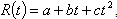 ,
,  and c are constants. Such that
 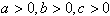 . Here a stands for the initial demand rate and b for the positive trend in demand.(ii) The production rate Say
 , where
  . A fraction
  ,
,  of the on-hand inventory deteriorates per unit time. (iii) The lead-time is zero and shortages are not allowed.(iv) Unit holding cost
  per unit time and unit deterioration cost
  per unit time are known and constants.(v)
  is the total average cost for the production cycle and
  is the stock level reached in the cycle.(vi) The set up cost is not considered in this model because it is taken to be fixed for the whole cycle time.(vii) Planning horizon is finite.
3. Mathematical Formulation and Solution
Let q be the inventory level at any time  . The differential equations governing the system in the interval
  are
are 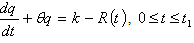 | (1) |
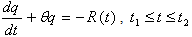 | (2) |
The stock level initially is zero. Production begins just after t=0, continues up to  and stops as soon as the stock level becomes S. Then the inventory level decreases due to demand and deterioration both till it becomes zero at
  . The cycle then repeats itself. Our objective is to determine the optimum values of
  and
and  . The intensity of deterioration is very low initially but it increases with time. However, it remains bounded for
  Using the value of
  , the two equations (1) and (2) take the form
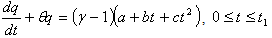 | (3) |
and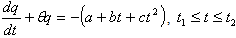 | (4) |
The solution of equation (3) with initial conditions is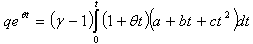 or
or 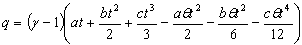 | (5) |
Neglecting the powers of  greater than 1.Similarly, the solution of equation (4) also is (neglecting the powers of
  greater than 1)
 or
or 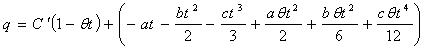 | (6) |
For 
 | (7) |
From (6) and (7) we get the relation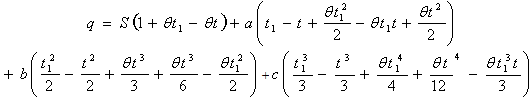 | (8) |
Using the condition  for
for  in equation (8), we get
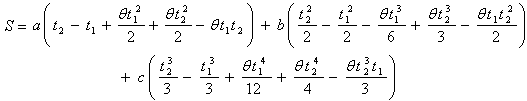 | (9) |
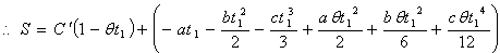
Now the average holding cost becomes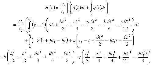 Now substituting the value of from (9) and simplifying we get
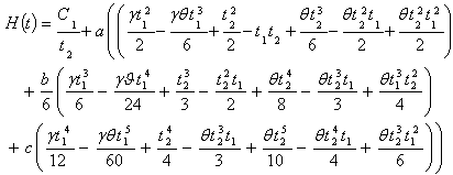 | (10) |
The average cost due to deterioration in the total cycle time is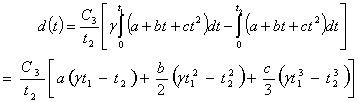 | (11) |
From (10) and (11) the total average cost of the inventory I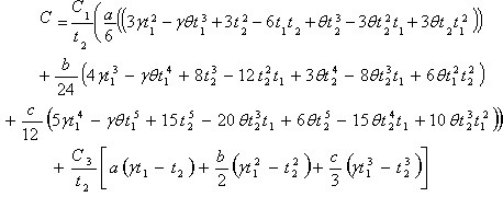 | (12) |
By putting  (where
  ) in equation (12), we get
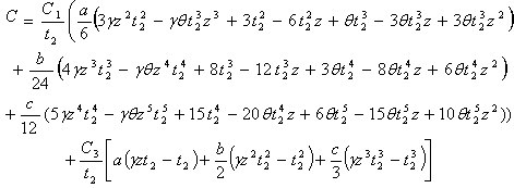 | (13) |
For calculating the optimum value of C we differentiate it partially with respect to  and equate them to zero. Thus we get the following equation:-
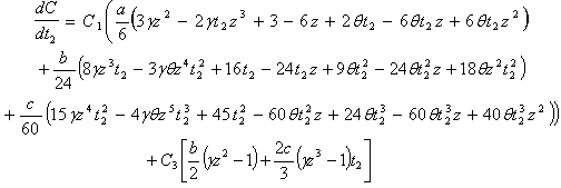 | (14) |
This equation gives us the optimum value of  which, when substituted equation (13), give the total average cost, provided
  . Equation (14) is highly non-linear in
  and cannot be solved analytically. This equation, therefore, can be solved by some suitable numerical method like Newton-Raphson, and optimal value of
  can be obtained. This optimal value of
  gives the minimum cost of the system in question. We have solved this equation on computer for a set of values of the parameters with the help of Newton-Raphson method. A numerical example is given below as an illustration.
3.1. Example-1
Let θ=0.02,  =2.0, z=0.7, C1=5.0, C3=60, a=200, b=40, c=10 in suitable units.The solution for optimal values of
 and
and  is
is 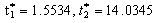 , which gives minimum average cost
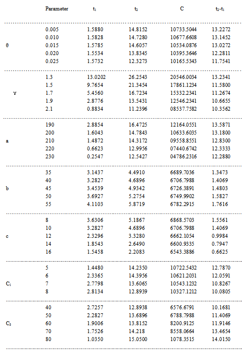
  Following are a number of tables representing the optimal values of
  ,
, and C as also the no-production interval
  .
.
4. Sensitivity Analysis
We have discussed the effects of the different parameters.(i) Increase in the value of  decreases the value of
  ,
, and C.(ii) Increase in the value of the parameter
 , decrease the values of
  ,
, and C.(iii) Increase in the value of holding cost
  increases the value of the cost
  ,
, and decreases the value of C.(iv) Increase in the value of deterioration cost
  increases the value of the cost
 and C. However the values of
  decrease. Increase in the value of a, decreases the value of C,
  ,
,  . Increase in the value of b, increases the values of
  ,
, and C. (v) Increase in the value of c, decreases the value of C,
  ,
,  .(vi) Keeping these variations in mind of the decision maker of the inventory system can control the parameters so as to optimize the objective function. The decision maker may control particularly the holding cost and the cost of deterioration for minimizing the total average cost.
 Table 1. Variations in parameters
 |
| |
|
5. Conclusions
In this article, a deterministic inventory model has been proposed for deteriorating item with quadratic demand rate, where shortages are not allowed. The goal of the paper is to incorporate the deterioration phenomenon together into an inventory model over a finite planning horizon. This paper investigates inventory-production systems where items follow constant deterioration. The objective is to develop an optimal policy that minimizes total average cost. The quadratic demand technique is applied to control the problem in order to determine the optimal production policy, holding cost and cost of deterioration.
References
| [1] | Goswami, K. Chaudhuri, an EOQ model for deteriorating items with shortages and a linear trend in demand, J. Opl. Res. Soc. 42 (1991) 1105-1110. |
| [2] | A. Bradshaw, Y. Erol, Control policies for production inventory systems with bounded input, Int. J. Sys. Sci. 11 (1980) 947-959. |
| [3] | B. Hamid, Replenishment schedule for deteriorating items with time proportional demand. J. Oper. Res. Soc.40 (1989) 75-81. |
| [4] | H. Wee, Economic production lot size model for deteriorating items with partial back ordering, Comput. Ind. Eng. 24 (1993) 449-458. |
| [5] | K. Heng, J. Labban, R. Linn. An order level for deteriorating items with partial back ordering, Comput. Ind. Eng. 20 (1991) 187-197 |
| [6] | T.M. Murdeshwar Inventory replenishment policy for linearly increasing demand considering shortages- an optimal solution. J.OplRes.Soc.39, (1988) 687 692 |
| [7] | U. Haiping, H. Wang, An economic ordering policy model for deteriorating items with time proportional demand, Eur. J. Oper. Res. 46 (1990) 21-27. |
| [8] | W.A. Donaldson Inventory replenishment policy for a linear trend in demand- an analytical solution. Opl Res. Q. 28,(1977) 663-670. |
| [9] | W.I Zangwill (1966) A deterministic multi-period production scheduling model with backlogging. Mgmt. Sci. 13, (1966) 105-119. |
| [10] | S.K.Sahu ,P.K.Sukla,A note for weibul deteriorating model with time varying demand and partial back-ordering.Acta Cienia Indica,vol,xxxiv M,No,4,(2008) 1673-1670. |
 Abstract
 Reference
 Full-Text PDF
 Full-Text HTML