Gobinda Chandra Panda1, Satyajit Sahu1, Manoj Kumar Meher2
1Dept of Mathematics, Mahavir Institute of Engineering and Technology, Bhubaneswar, Odisha
2Department of Computer science, Madanabati public School, Sambalpur, Odisha
Correspondence to: Gobinda Chandra Panda, Dept of Mathematics, Mahavir Institute of Engineering and Technology, Bhubaneswar, Odisha.
| Email: |  |
Copyright © 2012 Scientific & Academic Publishing. All Rights Reserved.
Abstract
In this paper, the two warehouse inventory problem for deteriorating items with exponentially increasing time demand rate and shortages is considered. Here existing storage is known as own warehouse OW and the other is hired on rental basis known as rented warehouse RW. The model allows different levels of item deterioration in both warehouses. Here replenishment rate is finite. The stock is transferred from RW to OW in continuous release pattern and the associated transportation cost is taken into account. Shortage in OW is allowed and excess demand is backlogged. An attempt is made to incorporate the different preservation facilities in own and rented warehouses for deteriorating items with exponentially time dependent demand. It is also assume that the preservation facility in RW is better than OW. For the general model, we give the equations for the optimal policy and cost function and we discuss some special case. A numerical example is given to illustrate the solution procedure of the model.
Keywords:
Two Warehouse Inventory Model, Own Warehouse, Rented Warehouse, Stock
Cite this paper:
Gobinda Chandra Panda, Satyajit Sahu, Manoj Kumar Meher, "Equation Chapter 1 Section 1A Two Warehouse Inventory Model for Deteriorating Items with an Exponential Demand and Shortage", American Journal of Operational Research, Vol. 2 No. 6, 2012, pp. 93-97. doi: 10.5923/j.ajor.20120206.02.
1. Introduction
In the busy markets like super market, corporation market, municipality market etc., the storage area of items is limited. When an attractive price discount for bulk purchase is available or the cost of procuring goods is higher than the other inventory related cost or demand of items is very high or there are some problems in frequent procurement, management decide to purchase a large amount of items at a time. These items cannot be accommodated in the existing store house (viz. the Own Warehouse, OW) located at busy market place. In this situation, for storing the excess items, one (sometimes more than one) additional warehouse (viz., rented warehouse, RW) is hired on rental basis, which may be located little away from it. We assume that the rent (holding cost for the item) of RW is greater than OW and hence the items are stored first in OW and only excess stock is stored in RW, which are emptied first by transporting the stocks from RW to OW in a continuous release pattern for reducing the holding cost. The demand of items is met up at OW only.The two warehouse inventory model has been considered by various authors in recent years. This type of model was discussed by Hartely,Sarma[2] developed model with finite production rate, but without shortages Dave[3] discussed the inventory models for finite and infinite rate of replenishment rectifying the errors for the model given by Sarma[2] and gave a complete solution, further Goswami and Chaudhuri[4] considered the models with or without shortages taking linearly increasing time dependent demand correcting and modifying the assumptions of Goswami and Chaudhuri [4], Bhunia and Maiti(9) analysed the same inventory model and graphically presented a sensitivity analysis on the optimal average cost and the cycle length for the variations of the demand parameters, in all these models only the cases of non deteriorating items were discussed.In reality, many physical goods deteriorated due to dryness, damage, spoilage, vaporisation etc. over time during their normal storage period. The deterioration also depends on preserving facility and environmental conditions available in warehouse and hence different warehouse may have different deterioration rates. Assuming the deterioration in both warehouses, Sarma[2] presented a model with infinite replenishment rate and shortage. Also Pakkala and Achary[7]developed the two warehouse model for deteriorating items with finite replenishment and shortage taking time as discrete and continuous variable respectively. In all models discussed in these papers, the demand was taken as uniform; the scheduling period (cycle length) was supposed to be constant and the transportation cost for transferring the stocks from RW to OW, was not taken into account. Bhunia and Maiti[9] modified and studied a two-warehouse inventory model for deteriorating items considering linearly time-dependent demand and shortages (for single period).We have also reviewed the article developed by Panda and Sahu[10]and the article Panda, Sahoo and Sukla[11] for developing idea to preparing this manuscript.In this paper we have studied a two storage facilities inventory model for deteriorating items with the following characteristics, Demand is exponentially increasing with time shortage are allowed and excess demand over supply is backlogged stock is transferred from RW to OW under a continuous release pattern and the transportation cost is taken into account. The deterioration rates are a constant but different in RW and OW due to preservation procedures. The scheduling period is not taken to be constant but variable. Some special cases of the general model are discussed. A numerical example is given in order to illustrate the solution to the model. Also, a sensitivity analysis has been performed to study the variation of the optimal stock level of RW and total cost per unit of time in the inventory system with respect to some input parameters.
2. Assumptions and Notations
The following notations are used in the proposed model:R(t)=demand rate which is an exponential function of time t ( -e-at , , a > 0).S = total highest stock level at RW and OW at the beginning of the cycle.T=cycle length, a variable of the system.W(L2=identifies an inventory system with two storage facilities.F, H(F>H) = holding costs for items in the RW and OW respectively.C2=shortage cost per unit of item per unit of time in shortage.C3=transportation cost per unit of item moved from RW to OW.A=replenishment cost (ordering cost) per replenishment with different values for L2 system, where A1+A2 for L2-system, A2 being the additional replenishment cost due to the transportation cost, loading and unloading costs for excess items in rented warehouse.C=cost of deteriorated unit.α, β=deterioration rates in OW and RW respectively , 0< α, β<1Q0(t), Qr(t)=inventory level in OW and RW at any instant t respectively.Q(t) = inventory level at OW during the period of shortage accumulation.To develop the model, the following assumptions are imposed:(1) Replenishment rate is infinite.(2) Lead time is zero.(3) Shortages are allowed and excess demand at OW, if any, is backlogged.(4) The rented warehouse RW has unlimited capacity.(5) The goods of OW are consumed only after consuming the goods kept in RW.(6) For L2-system, the initial inventory levels at RW and OW are S-W and W respectively where S is a variable , but W is constant.
3. Model Description and Analysis
During the interval (0,t1) the inventory S-W in RW gradually decrease due to demand and deterioration and it vanish at t=t1. In OW, the inventory W decreases during (0,t1) due to deterioration only and during (t1, t2) due to both demand and deterioration. At t=t1 the inventory in OW reaches zero and there after the shortage are allowed to occur down during the interval (t2,T). The shortage quantity is supplied to customers at the beginning of the next cycle. Hence, 0121 and T which minimize the total cost per unit time of the inventory system and subsequently to obtain the corresponding optimal values of S and the total cost per unit time.The stock depletion at RW during (0≤ t ≤ t1 )is mainly due to demand and partly due to deterioration of the items which are disposed continuously as they come to the selling point. Therefore, the rate of change of stock at RW at any instant t (due to stock depletion) is equal to the sum of demand and deterioration at that time. Hence the inventory level Qr(t) ( as figure-1 ) at RW satisfies the differential equations.  | (1) |
With the boundary condition that  . Due to the assumptions made also have
 | (2) |
During 0≤ t ≤ t1, as the demand is meet from RW, the stock at OW decreases due to deterioration only. Hence, the rate of change of stock at OW at any instant t(0≤ t ≤ t1) is equal to the deteriorations at that time. Again the stock depletion at OW during t1 ≤ t ≤ t2 is due to demand and deterioration of the items. Therefore the inventory level Q0(t) ,during 0≤ t ≤ t2 ,at OW satisfies the differential equations: | (3) |
 | (4) |
Solution of equation (1) is given by | (5) |
According to physical consideration imply that Q0(t) is continuous at t=t1.The solution of equation (3) and (4) are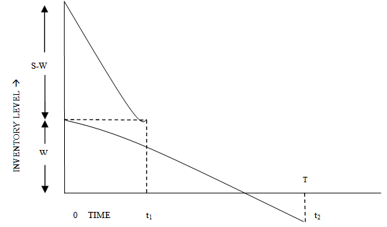 | Figure 1. The inventory situation in RW and OW |
 | (6) |
 | (7) |
Now using the continuity of  at t=t1, we have
 | (8) |
Which gives the solution that | (9) |
From equation (2) we have | (10) |
The total amount of deteriorated items in RW and OW are respectively and
and  Hence the total amount of deteriorated items in both RW and OW is
 | (11) |
The mean stock level of inventory carried in RW and OW multiplied by the time carried aregiven respectively by | (12) |
And | (13) |
The total amount of shortage for the entire cycle is 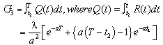 | (14) |
The total cost of the system during the interval (0,T) is thus given by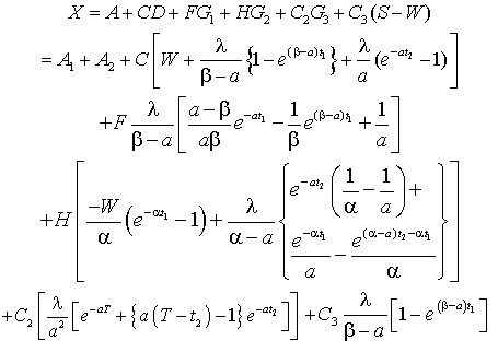 | (15) |
And its total cost per unit time is | (16) |
and t2 is approximately related to t1 through equation (9).The optimal values of t1 and T for minimum total cost per unit time is any solution of thesystem | (17) |
Which also satisfies the conditions Where the suffix denote the partial derivatives of the function with respect to those suffixes.Using these optimal values of t1 and T the optimal values of S and the minimum average costcan be obtained from (10) and (16) respectivelyEquation (17) are equivalent to
 | (18) |
The first part of equation (18) can be written as The second part of equation (18) can be written as
 The system of equations (18) has not a unique solution in t1,T so after having all its solutions, we must reject the non-admissible ones and check the remaining in order to find the optimal ti, T values.
4. Numerical Example
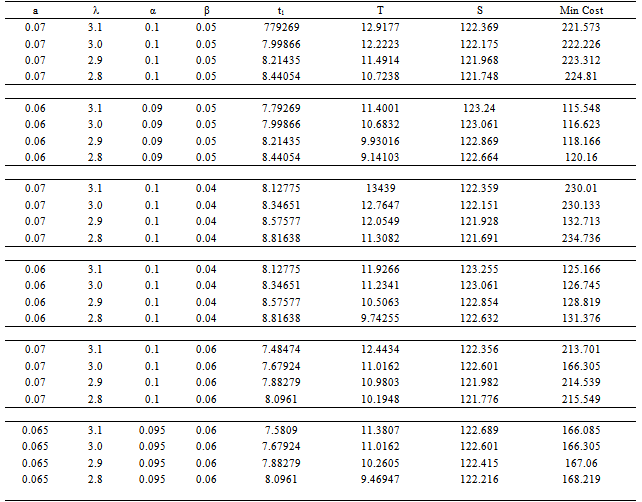
The developed model is illustrated by the following numerical example.Let C=2, H=0.5, F=1, C2=4, A1=150, A2=50, C3=0.2,W=100 in appropriate units.By taking the appropriated expression for t2 in equation (9), the optimum values of S and T along with minimum average cost and the boundary has been calculated for different values of demand parameter and a and deterioration parameter α and β using proper decision procedure and equation (18). Results are shown in Table-1.The following table represents the different cost with the total cost present in the paper by changing the different parameters percentage wise i.e. increased and decreased to the original value of the parameter given in the paper by numerical study.Table 1. Optimal Solution Obtained for the Numerical Example
 |
| |
|
In the above table we have analyzing the different parameters used in the research paper i.e. by the help of numerical study by using the software MATHEMATICA. The analysis is based open the sensitivity analysis i.e. we have increased and decreased in the original value of the parameters used in the paper and getting the numerical value i.e. present in the above table.
5. Sensitivity Analysis
We will now study the sensitivity analysis of the optimal solution to changes in the values of the different parameters associated with the inventory system in example. The results are showing in Table -1. A careful study of sensitivity analysis of Table-1 reveals the following points. It is clearly seen that from the above table, the changes in parameters a, , α, β respectively. We are getting the changes in T, S, and Min Cost respectively. Where T=cycle length and S = total highest stock level at RW and OW at the beginning of the cycle.
6. Conclusions
In this paper, an attempt is made to incorporate the different preservation facilities in own and rented warehouses for deteriorating items with exponentially time dependent demand. It is also assume that the preservation facility in RW is better than OW.As the rate of demand is assumed to be time dependent so the entire cycle over the first period cannot repeat after the cycle length T. It can be subsequently repeated with the changed value of the constant ‘’ and ‘a’ computed by the demand function. (where T associated value of the previous period)As the demand for the food grains increases with time, the present model is applicable for food grains like paddy, wheat etc. It is also applicable to other items whose demand is dependent exponentially with time. The proposed model assumes that the selling price and advertising level is reflected in the constant terms and a of the demand. As these are under the decision maker’s control the development of a more general inventory model, explicitly incorporating these variables, would then be appropriate.
References
| [1] | Hartly V R (1976). Operations Researcg – A managerial Emphasis, Chapter 12 Good Year, Santa Monica, CA, PP 315-317. |
| [2] | Sarma KVS (1983) A deterministic inventory model with two level of storage and a optimum release rule. Opsearch 20: 175-180. |
| [3] | Dave u (1988). On the EOQ models with two levels of storage. Opserarch 25 : 190-196. |
| [4] | Goswami A and Chaudhuri KS (1992) An economic order quantity model for items with two levels of storage for linear trend in demand J Opl Res Soc 43; 157-167. |
| [5] | Bhunia AK and Maiti M (1994) A two warehouse inventory for a linear trend in demand. Opsearch 31: 318-329. |
| [6] | Sharma KVS(1987) A deterministic order - level- inventory model for deteriorating items with two storage facilities Eur J Opl res 29: 70-72. |
| [7] | Pakkala TPM and Acharya KK (1992) Discrete time inventory model for deteriorating items with two storage facilities . Eur J Opl Res 29; 90-103. |
| [8] | Pakkala TPM and Achary KK (1992) : A deterministic inventory model for deteriorating items with two warehouses and finite replenishment rate . Eur J Opl Res 57: 71-76. |
| [9] | Bhunia AK and Maiti M. (1998) : A two warehouse inventory model for deteriorating items with a linear trend in demand and shortages. J of the Opl Res Society 49: 287-292. |
| [10] | Panda G.C and Sahu S.K (2007) :Weibull Deterioration and delay in payments .SCMS Journal of Indian Management. Vol.IV, No.IV,pp.68-79. |
| [11] | Panda Gobinda Chandra ,Sahoo S and Sukla P.K (2012): Analysis of Constant Deteriorating Inventory Management with Quadratic demand rate. Accepted in American Journal of Operations Research. Vol.2,No.6,2012. |
 Abstract
 Reference
 Full-Text PDF
 Full-Text HTML