1. Introduction

In conventional inventory models, uncertainties are treated as randomness and are being handled by applying the probability theory. However, in certain situations uncertainties are due to fuzziness, and such cases are dilated in the fuzzy set theory which was demonstrated by Zadeh in[12]. Kauffmann and Gupta[1] provided an introduction to fuzzy arithmetic operation and Zimmermann[4] discussed the concept of the fuzzy set theory and its applications.

Considering the fuzzy set theory in inventory modeling renders an authenticity to the model formulated since fuzziness is the closest possible approach to reality. As reality is imprecise and can only be approximated to a certain extent, same way, fuzzy theory helps one to incorporate uncertainties in the formulation of the model, thus bringing it closer to reality.

Park[10] applied the fuzzy set concepts to EOQ formula by representing the inventory carrying cost with a fuzzy number and solved the economic order quantity model using fuzzy number operations based on the extension principle. Vujosevic et al.[15] used trapezoidal fuzzy number to fuzzify the order cost in the total cost of the inventory model without backorder, and got fuzzy total cost. Yao and Lee [7] introduced a backorder inventory model with fuzzy order quantity as triangular and trapezoidal fuzzy numbers and shortage cost as a crisp parameter. Gen et al.[14] expressed their input data as fuzzy numbers, and then the interval mean value concept was introduced to solve the inventory problem. Chang et al.[20] considered the backorder inventory problem with fuzzy backorder such that the backorder quantity is a triangular fuzzy number.

Chang[21] discussed the fuzzy production inventory model for fuzzify the product quantity as triangular fuzzy number. Lee and Yao[5] proposed the inventory without backorder models in the fuzzy sense, where the order quantity is fuzzified as the triangular fuzzy number. Yao et al.[9] assumed to be the order quantity and the total demand rate as triangular fuzzy numbers and obtained the fuzzy inventory model without shortages. Wu and Yao[11] fuzzified the order quantity and shortage quantity into triangular fuzzy numbers in an inventory model with backorder and they obtained the membership function of the fuzzy cost and its centroid. Yao and Chiang[8] considered the total cost of inventory without backorder. They fuzzified the total demand and cost of storing one unit per day into triangular fuzzy numbers and defuzzify by the centroid and the signed distance methods. Dutta et al.[17] developed a model in presence of fuzzy random variable demand where the optimum is achieved using a graded mean integration representation. Chang et al.[3] developed the mixture inventory model involving variable lead-time with backorders and lost sales. First they fuzzify the random lead-time demand to be a fuzzy random variable and then fuzzify the total demand to be the triangular fuzzy number and derive the fuzzy total cost. By the centroid method of defuzzification, they estimate the total cost in the fuzzy sense. Wee et al.[6] developed an optimal inventory model for items with imperfect quality and shortage backordering. Lin[23] developed the inventory problem for a periodic review model with variable lead-time and fuzzified the expected demand shortage and backorder rate using signed distance method to defuzzify. Roy and Samanta[2] discussed a fuzzy continuous review inventory model without backorder for deteriorating items in which the cycle time is taken as a symmetric fuzzy number. They used the signed distance method to fuzzify the total cost. Gani and Maheswari[16] developed an EOQ model with imperfect quality items with shortages where defective rate, demand, holding cost, ordering cost and shortage cost are taken as triangular fuzzy numbers. Graded mean integration method is used for defuzzification of the total profit. Ameli et al.[13] developed a new inventory model to determine ordering policy for imperfect items with fuzzy defective percentage under fuzzy discounting and inflationary conditions. They used the signed distance method of defuzzification to estimate the value of total profit. Nezhad et al.[22] developed a periodic review model and a continuous review inventory model with fuzzy setup cost, holding cost and shortage cost. Also they considered the lead-time demand and the lead-time plus one period’s demand as random variables. They use two methods in the name of signed distance and possibility mean value to defuzzify. Uthayakumar and Valliathl[19] developed an economic production model for Weibull deteriorating items over an infinite horizon under fuzzy environment and considered some cost component as triangular fuzzy numbers and using the signed distance method to defuzzify the cost function.

In this paper, an inventory model for deteriorating items with shortages is considered where demand, holding cost, unit cost, shortage cost and deterioration rate are assumed as a triangular fuzzy numbers. For defuzzification of the total cost function, Graded Mean Representation, Signed Distance and Centroid methods are used. By comparing the results obtained by these methods, we get the better one as an estimate of the total cost in the fuzzy sense.

2. Preliminaries

In order to treat fuzzy inventory model by using graded mean representation, signed distance and centroid to defuzzify, we need the following definitions.

Definition 2.1 (By Pu and Liu[18, Definition 2.1]). A fuzzy set on is called a fuzzy point if its membership function is

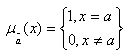(1)

where the point a is called the support of fuzzy set .

Definition 2.2 A fuzzy set where and a < b defined on , is called a level of a fuzzy interval if its membership function is

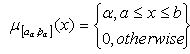(2)

Definition 2.3 A fuzzy number where a < b < c and defined on , is called a triangular fuzzy number if its membership function is

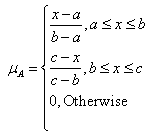(3)

When , we have fuzzy point

The family of all triangular fuzzy numbers on is denoted as

.

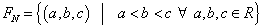The -cut of is.

Where and are the left and right endpoints of.

Definition 2.4 If is a triangular fuzzy number then the graded mean integration representation of is defined as

with .

. (4)

Definition 2.5 If is a triangular fuzzy number then the signed distance of is defined as

(5)

Definition 2.6 The centroid method on the triangular fuzzy number is defined as

(6)

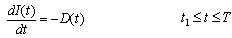
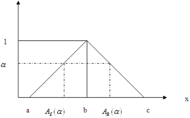Figure. -cut of a triangular fuzzy number

3. Assumptions and Notations

The mathematical model in this paper is developed on the basis of the following assumptions and notations.

3.1 Notations

(i) is the demand rate at any time per unit time.

(ii) is the ordering cost per order.

(iii) is the deterioration rate,

(iv) is the length of the Cycle.

(v) is the ordering Quantity per unit.

(vi) → is the holding cost per unit per unit time.

(vii) is the shortage Cost per unit time.

(viii) is the unit Cost per unit time.

(ix) → is the total inventory cost per unit time.

(x) is the fuzzy demand.

(xi) is the fuzzy deterioration rate.

(xii)is the fuzzy holding cost per unit per unit time.

(xiii) is the fuzzy shortage Cost per unit time.

(xiv) is the fuzzy unit Cost per unit time.

(xv) is the total fuzzy inventory cost per unit time.

(xvi) is the defuzzify value of by applying Graded mean integration method

(xvii) is the defuzzify value of by applying Signed distance method

(xviii) is the defuzzify value of by applying Centroid method.

3.2 Assumptions

(i)→Demand is assumed to be an increasing function of time i.e. where and are positive constants and .

(ii)→Replenishment is instantaneous and lead-time is zero.

(iii)→Shortages are allowed and fully backlogged.

4. Mathematical Model

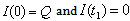
Let be the on-hand inventory at time t with initial inventory . During the period[0, ] the on-hand inventory depletes due to demand and deterioration and exhausted at time . The period[, T] is the period of shortages, which are fully backlogged. At any instant of time, the inventory level is governed by the differential equations.

4.1. Crisp Model

(4.1)

With .

(4.2)

With .

The solution of equation (4.1) and (4.2) is given by

(4.3)

and

(4.4)

By using , we have

(4.5)

Now, (4.3) becomes

(4.6)

(Neglecting higher powers of ).

Total average no. of holding units () during period[0, T] is given by

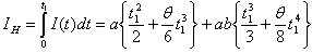(4.7)

Total no. of deteriorated units () during period[0, T] is given by

Total Demand

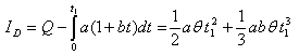(4.8)

Total average no. of shortage units during period[0, T] is given by

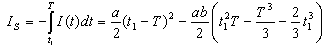(4.9)

Total cost of the system per unit time is given by

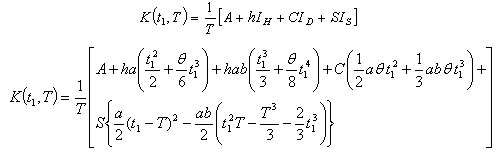(4.10)

4.2. Fuzzy Model

Due to uncertainly in the environment it is not easy to define all the parameters precisely, accordingly we assume some of these parameters namely may change within some limits.

Let are as triangular fuzzy numbers.

Total cost of the system per unit time in fuzzy sense is given by

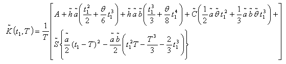(4.11)

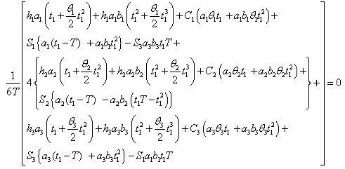
We defuzzify the fuzzy total cost by graded mean representation, signed distance and centroid methods.

(i) By Graded Mean Representation Method, Total Cost is given by

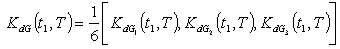Where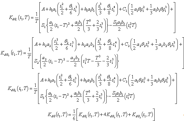

(4.12)

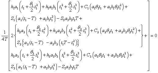
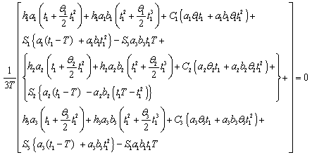
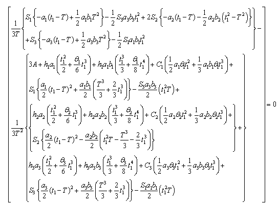
To minimize total cost function per unit time, the optimal value of and can be obtained by solving the following equations:

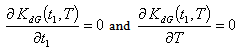(4.13)

Equation (4.13) is equivalent to

(4.14)

and

(4.15)

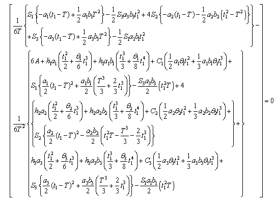
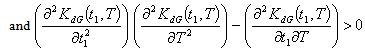
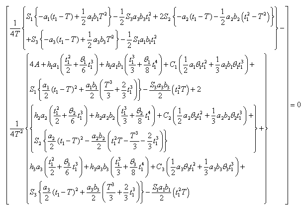
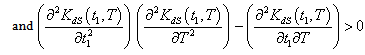
Further, for the total cost function to be convex, the following conditions must be satisfied

(4.16)

(4.17)

The second derivatives of the total cost function are complicated and it is very difficult to prove the convexity mathematically. Thus, the convexity of total cost function has been established graphically, (Figure (A)).

(ii) By Signed Distance Method, Total cost is given by

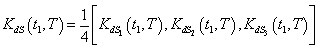Where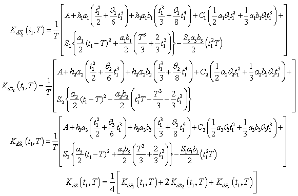

(4.18)

The total cost function has been minimized following the same process as has been stated in case (i).

To minimize total cost function per unit time , the optimal value of and can be obtained by solving the following equations:

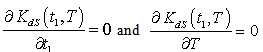(4.19)

Equation (4.19) is equivalent to

(4.20)

and

(4.21)

Further, for the total cost function to be convex, the following conditions must be satisfied

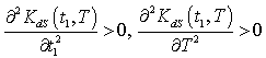(4.22)

(4.23)

The second derivatives of the total cost function are complicated and it is very difficult to prove the convexity mathematically. Thus, the convexity of total cost function has been established graphically, (Figure (B)).

(iii)By Centroid Method, Total cost is given by

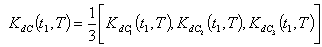Where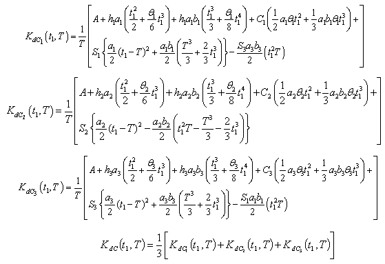

(4.24)

The total cost function has been minimized following the same process as has been stated in case (i).

To minimize total cost function per unit time , the optimal value of and can be obtained by solving the following equations:

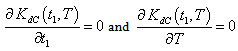(4.25)

Equation (4.25) is equivalent to

(4.26)

and

(4.27)

Further, for the total cost function to be convex, the following conditions must be satisfied

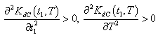(4.28)

(4.29)

The second derivatives of the total cost function are complicated and it is very difficult to prove the convexity mathematically. Thus, the convexity of total cost function has been established graphically, (Figure (C)).

5. Numerical Example

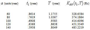
Consider an inventory system with following parametric values.

Crisp Model, /order, /unit, Rs. 5/unit/year, units/year, units/year, /year, Rs 15 /unit/year.

The solution of crisp model is

Rs 404.3429, =. 7149 year, T = .9636 year.

Fuzzy Model,

The solution of fuzzy model can be determined by following three methods.

By Graded Mean Representation Method, we have

1. When all are triangular fuzzy numbers

= Rs 414.6096, = .6908 year, T= .9383 year.

2. When are triangular fuzzy numbers

= Rs 406.9852, =. 7135 year, T = .9560 year.

3. When are triangular fuzzy numbers

= Rs 405.5274, =. 7115 year, T= .9596 year.

4. When and are triangular fuzzy numbers

= Rs 405.2250, =. 7120 year, T = .9603 year.

5. When and are triangular fuzzy numbers

= Rs 404.8978, =. 7131 year, T = .9611 year.

By Signed Distance Method, we have

1. When all are triangular fuzzy numbers

= Rs 419.6059, =. 6797 year, T = .9266 year.

2. When are triangular fuzzy numbers

= Rs 408.2810, =. 7128 year, T= .9523 year.

3. When are triangular fuzzy numbers

= Rs 406.1163, =. 7093 year, T= .9576 year.

4. When and are triangular fuzzy numbers

= Rs 405.6640, =. 7106 year, T = .9587 year.

5. When and are triangular fuzzy numbers

= Rs 405.1742, =. 7122 year, T = .9599 year.

By Centroid Method, we have

1. When all are triangular fuzzy numbers

= Rs 424.5173, =. 6691 year, T = 9153 year.

2. When are triangular fuzzy numbers

= Rs 409.5606, =. 7121 year, T = .9487 year.

3. When are triangular fuzzy numbers

= Rs 406.7030, =. 7074 year, T = .9557 year.

4. When and are triangular fuzzy numbers

= Rs 406.1016, =. 7092 year, T = .9571 year.

5. When and are triangular fuzzy numbers

= Rs 405.4499, =.7113 year, T = .9587 year.

6. Sensitivity Analysis

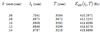
A sensitivity analysis is performed to study the effects of changes in fuzzy parameters , and on the optimal solution by taking the defuzzify values of these parameters. The results are shown in below tables.

Table 1. Sensitivity Analysis on parameter

Table1 indicates that as the value of increases, fuzzy cost increases significantly but and decreases drastically.

Table 2. Sensitivity Analysis on parameter

Table 2 indicates that as the value of increases, fuzzy cost increases regularly but and decreases gradually.

Table 3. Sensitivity Analysis on parameter

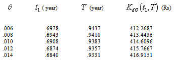
Table 3 indicates that as the value of increases, fuzzy cost increases slightly but and decreases gradually.

If we plot the total cost function with some values of and s.t. = .65 to 2 with equal interval = .84 to 1, then we get strictly convex graph of total cost function

given below.

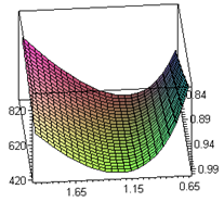Figure (A). Total Fuzzy Cost Vs. and

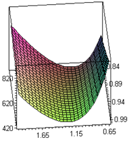Figure (B). Total Fuzzy Cost Vs. and

If we plot the total cost function with some values of and s.t. = .65 to 2 with equal interval = .84 to 1, then we get strictly convex graph of total cost function given below.

If we plot the total cost function with some values of and s.t. = .65 to 2 with equal interval = .84 to 1, then we get strictly convex graph of total cost function

given below.

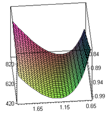Figure (C). Total Fuzzy Cost Vs. and

7. Conclusions

This paper presents a fuzzy inventory model for deteriorating items with allowable shortages in which demand is an increasing function of time. The demand, deterioration rate, inventory holding cost, unit cost and shortage cost are represented by triangular fuzzy numbers. For defuzzification, graded mean, signed distance and centroid method are employed to evaluate the optimal time period of positive stock and total cycle length T which minimizes the total cost. By given numerical example it has been tested that graded mean representation method gives minimum cost as compared to signed distance method and centroid method. A sensitivity analysis is also conducted on the parameters and to explore the effects of fuzziness.

Finding Suggest that the change in parameters and will result the change in fuzzy cost with some changes in and .With the increases values of these parameters will result in increase of fuzzy cost, but decreases and . Similarly with the decreases values of these parameters will result in decrease of fuzzy cost, but increases and .

A future study would be to extend the proposed model for finite replenishment rate, stock outs, which are partially backlogged, price dependent demand, stock dependent demand and many more.

ACKNOWLEDGEMENTS

The authors would like to thank anonymous referees for their valuable and constructive comments and suggestions that have led to improvement on the earlier version of the paper. The first author would like to acknowledge the support of the Research Grant No.: Dean(R/R&D/2012/917), provided by the University of Delhi, Delhi, India for conducting this research. The third author would like to thank University Grants Commission for providing Junior Research Fellowship vide letter No. JRF/AA/168/2010-11, 47126.