-
Paper Information
- Next Paper
- Previous Paper
- Paper Submission
-
Journal Information
- About This Journal
- Editorial Board
- Current Issue
- Archive
- Author Guidelines
- Contact Us
American Journal of Operational Research
2012; 2(5): 51-59
doi: 10.5923/j.ajor.20120205.02
Dynamic Structure to Define a Corporate Channel for Courier Companies
 Abstract
 Reference
 Full-Text PDF
 Full-Text HTML
Daniel Alexander Méndez Rey 1, Jorge Eduardo Ortiz Triviño 2
1Master of Industrial Engineering Faculty of Engineering National University of Colombia Bogotá, Colombia
2Department of Industrial and Systems Engineering, Faculty of Engineering National University of Colombia Bogotá, Colombia
Correspondence to: Daniel Alexander Méndez Rey , Master of Industrial Engineering Faculty of Engineering National University of Colombia Bogotá, Colombia.
| Email: |  |
Copyright © 2012 Scientific & Academic Publishing. All Rights Reserved.
The document presents a stochastic linear programing model, providing a network structure to meet corporate clients to courier companies as a strategy of upkeep and increment in revenue. By reviewing the state of art about location models in different outlets in retail businesses over time, we take a courier company to define a location model of retail sales points, based on major revenue customer, the result gives optional strategies for network structure, where the model outputs are validated under changes in demand and network capacity in different scenarios, generating strategic options to be implemented in companies with the same characteristics. The project finds a form to eliminate the subjectivity that exists in the decision-making with location sales points problems in retail services companies.
Keywords: Retail, Location and Stochastic Linear Programming
Cite this paper: Daniel Alexander Méndez Rey , Jorge Eduardo Ortiz Triviño , "Dynamic Structure to Define a Corporate Channel for Courier Companies", American Journal of Operational Research, Vol. 2 No. 5, 2012, pp. 51-59. doi: 10.5923/j.ajor.20120205.02.
Article Outline
1. Introduction
- When a company begins a growth process, where its organizational approach is oriented to attend their customers through a sale’s point network, sell their products and/or services, they’ll come to the following question, what would be the ideal structure of the network, about quantity and location of self-sale’s points and franchises to maintain their clients and generate new revenue?In present times, this case has taken strength by having companies dedicated to perform consults to define ideal channel strategies for every type of business, under the premise: "Customer Satisfaction", this is an approach that strives to move an entire company to find new customer needs and participate actively in their satisfaction[1].However, companies have based their strategies in the search of profit without focusing on what really generates it, the client[1], from the 60's we can find models that begin the search for the best location for retail points, with the goal of eliminating the subjectivity of decisions of this type, oriented at the discretion who takes it, which have evolved until eliminating this subjectivity.Within the literature review we can find that this type of analysis on the market can cost around 100 to 200 million pesos, depending on the reach that we need, this value was provide by the base company for this model, who were in the bidding process for performing this review of channel strategy.In particular, this type of analysis is always trying to locate potential market access and penetration characteristics, this practice is being developed in courier companies that establish a network to cover their clients in a national basis, in the particular case of the project, working on a strategy of upkeep and diversification of actual customers, with the goal of maintaining of Pareto customers, where we define the strategies for satisfying them regarding their own retail points, franchises and collection circuits.The project scope is the definition of how many and where by municipalities should there be new owned sale points, franchises and collection circuits, finding strategies to expand the current network. To this purpose, we select a Pareto customer on which the company sees major revenues and analyses their needs for access to the network, thus generating the target location for the company.After doing the previous selection of the objective client to study, we proceed to identify his characteristics allowing us to find out where should a courier network be implemented, by taking into account all the possible locations the customer has access to, which are more than 300 municipalities and each one having different office locations on them. Afterwards we establish the municipalities where the study is to take place; we proceed to find out how is the state of the company’s network on these sites, generating arrays as the model’s parameters. This leads us to defined a lineal programing model with stochastic processes which focus on the client’s demand, allowing us to establish an ideal network structure, focused under the strategic options that the company should pursue in order to guarantee customer satisfaction.From the model result, we establish the need to generate optional scenarios, defining the strategic options given by the company, through three different scenarios, in which we monitor an initial profit (Revenues vs. network cost) on each, giving the necessary tools for the decisions to take. Lastly, we validate the results, establishing the network’s benefits, that the company will have in other to commercialize their products and services.
2. Companies’ Retail Points Locations
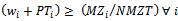
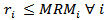
- As a fundamental principle for the growth of a company oriented to the generation of revenue, involving a set of strategies allowing the upkeep and development of this trough time where most of its revenue is perceived from their sales points, by selling their products or providing a service, the company is forced to analyse where to locate these retail points, guaranteeing their participation in the objective market.Trough studies done by SBA (Small Business Administration)[2], poor location of retail points could generate problems of capital shortage and eventually trigger a company’s down fall. On the other hand, poor location can be compensated with a good marketing strategy and / or promotions (bargains/deals), which would represent higher expenses for the company affecting the amount of profit it makes.The decision in where these locations should be situated is mainly motivated by:Start of a new business: This makes reference to the creation of a new company or a new business line which is in need of having retail points in order to participate in the objective market.Business growth: We define expansion as the need to be participating of the market, trough the network expansion allowing the increment of revenue and aiming to generate more profit, keeping in mind the possible need to relocate as the behaviour dictates.
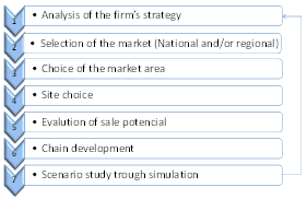 | Figure 1. Decision making process for the location of retails points |
3. Sales Points Location Model: State of Art
- As we mentioned before, retail companies should focus their efforts to successfully locate their retail points, because it is a vital point as a profitability model for the company. For this propose models have been designed over time trying to ease the decision making on this field, next we’ll present some cases
3.1. Check List Method
- This method was first propose be seen Applebaum (1965)[2], who tried to provide a procedure for the information evaluation related with the locations potential. From here, the factor check list is created which is used by the company with the objective to place retail locations according to the strategy option which are a priority in the development or their action plans. Some categories within in the check lists are: The Company’s strategies, basic economic factors, politics and government, taxes, licenses, environmental laws, commodities, international factors, competences amongst others. However, this type of analysis can become a subjective one as it focuses in the personal preferences of the one making it, slanting the location of the sales points to particular criteria.
3.2. Weighted Location Model
- This model consists in the making on the relative evaluation of each factor involved in the decision making of the retail points location, it’s a variation of the check list that gives a mathematical support for the decision making. In general, it evaluates each location for the preselected factor; next we present a brief description of this model[2]: Step 1: Allocation of relative importance to evaluat each factors: (1) Not Important, (2) Important and (3) Very Important. This classification can vary depending on the criteria of the one who applies it.Step 2: Classification of possible places to evaluate, for each of criteria selected in relevance with the numeric qualification, a scale from 1 - n is defined, where 1 is low score until we reach n as highest possible score.Step 3: Score for each analysed location, generated trough the multiplication of step 1 and 2, for each place and criteria establishing a total by location and choosing the site with the highest score.
3.3. LMMD Model
- The LMMD model is a weighted location model that was proposed by Richard Davis and Howard Rudd (1983) who used an easy model that can be applied to any retail company through a decision array that involves[2]:• Classification of location criteria.• Weighted criteria with a subjective evaluation by the one making the array.• Given score under a set scale defined by experts.The main characteristics of this model are: (1) The use of Delphi appreciation to evaluated de criteria in each location (Experts scoring), (2) The implementation process is short and (3) Advanced mathematics knowledge is not necessary for the execution of the model. This model integrates model A and B which simplify scoring by taking into account Delphi appreciations trying to minimize the subjective level on the decision making.
3.4. Analogic Method
- This method was introduced by Cohen (1960) and Applebaum (1960, 1968), it is a subjective approach to evaluate[3]:• Similar sales points to the one desired to open, with the objective to know how analogous stores attract clients form different areas.• Form this information we estimate the possible locations for these sales points according to analysis previously made.This method is frequently use when a company doesn’t have the necessary studies to locate their offices and references the competition establishing as a given that analogous companies make other types of analysis.
3.5. Regression Model
- It is a more rigorous model which tries to combined the check list method and the analogous method trough a regression model that allows us to determine the factors that affect the profitability of a sales point in a specific locationThere are several investigations about regression for this type of model, however, the profit Y= f (L, S, M, P, C) is always defined as a lineal function, the (L) location, sales points characteristics (S), market characteristics (M), prices (P) and competition (C)[3].
3.6. Other Locations Models
- In general terms, a company that wants to locate sales points needs to answer two main questions: (1) How does the sales points should be located? and (2) How to locate a sales points network from de same company to prevent cannibalization of the market? (Gérard Cliquet 2008)[4].According to the first question several models have emerged of which we have mentioned some already:• Check list: Applebaum – 1966, Kane 1966 and Nelson 1958• The analog method: Applebaum – 1968• Proximal areal method (Mid-Point): Ghosh and McLafferty 1987• Polynomials of Thiessen and Dirichlet: Dirichlet 1850 and Thiessen 1911• Gravity Models: Converse 1949 and Huff 1964• Interaction Models: Nakanishi and Cooper 1974As to the second question we can find the next models:• MULTILOC: Achabal 1982• P-Media Approach: Weber 1909 and Cooper 1963• Combination model with MCI (Multiplicative Competitive Interaction): Nakanishi and Cooper 1974• Qualitative Approach based on administrative criteria: Durvasula 1992• Multi-objective approach: Pirkil 1987, Current and Storbeck 1963 and Kolly y Evans 1999
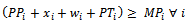
4. Present Intake Network
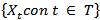
- After looking up the different options there are for the attention point’s locations, we can see the structure of the selected company to generate the proposed model, taking as a first step a diagnostic of the present network.By establishing a contract relationship with corporative clients trough a sales force, the client will have to his disposition the needed attention points in order to make their shippings, in this particular case if the client has offices in Bucaramanga, Cúcuta, Barranquilla, Cartagena, Cali, Pasto, Villavicencio, Tunja, Medellín, Manizales, Pereira, Armenia, Ibagué and Bogotá, he will have access to recollection circuits in their work place with a previous set time.Lastly, if the costumer is located in a place without this kind of service, he or she could come to one of the agencies that act as thirds that also cover the functions of intake of packages for corporative clients. The figure 2 clarifies what was mentioned before.
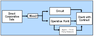 | Figure 2. Present structure of the intake network |
5. Inputs Model Information
- With the goal to determine the sufficient information for the development of the model, next we will present how the client on which the analysis is done, is selected, in order to determine the usage of the company’s services during the specific year, as well as other information needed for the development of the model.
5.1. Client Selection
- For the development of the project is necessary to select a client by whom we would try to improve the access level when it comes to the intake of his shippings on the present network; for this we took into account the revenue during the reference year and we selected the client with the major participation, this client is responsible for 4.53% of the company’s revenue reflected by 699.441 shipments done.With the objective to validate the model’s result, we determined the demand during 3 years, like this: (1) Client’s growth of 11% - (First year), (2) increment by 30% of the client’s demand (Second year) and (3) increment by 40% of the client’s demand (Third year).
5.2. Present Network Cost
- The present network cost for the attention of corporative clients, according to description given before, are established under the knowledge of the business by the company of the sector, where it’s defined that from the total network’s cost, 83% corresponds to infrastructure used for corporative clients.
5.3. Creation Cost of New Location or Third Party
- The company defines two options for the creation of new attention points, a self-point or through a third party agent, an allied network which fulfils with the location of the sales point and has an administration that assumes the functionality cost and defines a remuneration system with the company.
5.4. Client Structure
- First we chose a client established since the year 1991, which has offices, in 377 municipalities throughout the country and also has 625 different locations in given municipalities. The models that the courier company applies must guarantee access to the service offered to the client in all their locations.
6. Corporative Channel Attention Model
- The model is born from the need of expansion of a courier company that wants to change the strategy of their corporative channel, based on the increase of revenue, but focusing on customer satisfaction keeping in mind a Pareto client, prioritizing present customers making it a growth strategy on current clients, that would later allow us to obtain new customers through the structure of the channel.According to the information gathered for the formulation of the project, next we will show the lineal programing model with stochastic processes for the customer demand, which as a result gives us strategies for the aperture of locations (own points or third party agents) and implementation of recollection circuits.
6.1. Model Structure
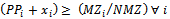
- The objective of this model is to widen the corporative client’s attention channel through minimizing costs for the channel, based on strategic options from the company for the aperture of locations (own points or third party agents) and implementation of recollection circuits.Index:i: Municipalities where the Pareto client is located t: Months of the year when the revision of the stochastic demand of the Pareto client is done.Variables:
 Number of new own attention points in the network per municipalities i
 Number of new third party attention points in the network per municipalities i
 Number of new recollection circuit per municipalities iParameters:
 Demand per municipalities i
 Attentions points of the Pareto client per municipalities iCPP: Monthly average capacity in present own locationsNMZ: Number of blocks strategic option of own locations NMZT: Number of blocks strategic option of third party locations
 Number of blocks per municipalities i where there are own pointsCT: Opening cost for new own sales point, first monthCA: Upkeep cost for own sales points, per monthCN: Opening cost for third party points, first monthCE: Upkeep cost for third party points, per monthCR: Average monthly cost for collection circuits MRM: Top number of collection circuits per municipalitiesPPi: Number of present own sales points per municipalities i-
 Number of present third party points per municipalities i
 Mathematical Model:Objective Function:Minimize the network cost:
  | (1) |
 | (2) |
 | (3) |
 | (4) |
 | (5) |
 | (6) |
 | (7) |
 | (8) |
 | (9) |
 | (10) |
 | (11) |
 | (12) |
6.2. Stochastic Demand Processes
- A stochastic process[5] is a family collection of random variables
 , ordered by t which usually indicates time, where
  is a random variable, namely for every moment of t, it has an independent random variable, in other words, we can establish that a stochastic process could be interpreted as a sequence of random variables whose characteristics vary along the index t.For the project case, the analysis demand for municipalities is an independent random variable, that shall be applied over one year,
  , which is estimated under a normal stochastic process that integrates Poisson and Weiner processes.According to research conducted by Girlich (1996) at the University of Leipzig in Germany[6], stochastic demand processes must first establish the domestic demand processes which can be approximated by special Gaussian processes and then review the single product or service model, through a Gaussian process, specifically Wiener processes as a demand process.First, to explain the particular process applied, we must define the cumulative demand.Definition 1: A stochastic demand process
  with
with , is a stochastic process with independent and homogeneous increments which has finite variances for each
 .
.  denotes the cumulative demand during the time interval
 . From the present definition, we specify two important stochastic demand processes.Compound Poisson demand process[6]: In products that have low demand, these demand occurs in
  in sizes
 , where
  denotes the random number of demand cases until t. We say that N is a Poisson process with the parameter
  if for the increments
  , it holds:(i)
 , are independent random variables.(ii)
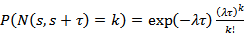
 | (13) |
 is equal to the cumulative demand in
 . We call D a compound Poisson demand process with the parameters
  and F if (i) and (ii) hold, and in addition:(iii)
  are independent and identically F-distributed integer-valued random variables which are independent from N.We say that D is a Poisson demand process if:
 | (14) |
 . For the expected cumulative demand in
  the following relations hold:
 | (15) |
 | (16) |
 of which is equal to the sum of the addends’ rate. The generalization to compound Poisson processes additionally needs a weighted sum of the distribution function that generates the next lemma.Lemma 1: For a sequence of n independent compound Poisson demand processes
  with parameters
  and
and , the distribution of
  is equal to the distribution of a compound Poisson demand process
  with parameters
  and
and  with:
with: | (17) |
 denote a normally distributed random variable with
 In some cases, for example when
 , we may describe the demand in
  by
by . A process
 , is a Gaussian process if its finite dimensional distributions are all normal. G is characterized completely by the main function
  and the covariance matrix with the elements
 For each finite set
 . We define a Gaussian demand process D as a Gaussian process with:
 In the special case
  , we speak of a Wiener demand process W. Therefore, it holds
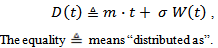 | (18) |
 with
with , be a sequence of independent copies of a stochastic demand process with
 . Then the sequence
  with:
with: | (19) |
 .Proof: A stochastic demand process has independent increments which are homogeneous. For that reason the conditions of a proposition given by M. Fisz[7] are fulfilled and thus easily verifies our assertion. The assumption of a sequence of independent copies may be weak.Theorem 2:
  with
with 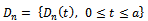 be a sequence of stochastic demand processes with the properties:(i)
 | (20) |
 there exists a
  with
with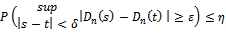 | (21) |
 converges to the Wiener process:
  .Normal approximation[6]: Now we apply the two limit theorems to compound Poisson demand processes.Corollary 1:
  be a sequence of independent copies of a compound Poisson demand process with parameters λ. And F. Then, for sufficiently a large n the following approximation holds.
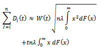 | (22) |
 be a sequence of independent compound Poisson demand processes with parameters
  and
and  , respectively. Then, for sufficiently large n the following approximation holds
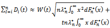 | (23) |
 and
and  are given by (17).Model Applying: In this particular case of the model, the demand per municipality is established under the following assumptions for (23):• λ is taken as a constant value, this estimated with the sample mean of the year available, this parameter is set to distribution population mean and the best estimation for this one is sample mean.•
 , Weiner distribution by definition as a standard normal distribution[7].• In order to check if in fact the variable X follows a normal distribution, we proceed to perform a goodness of fit test[8], according to available year information analysed, which shows the fit to this distribution, then comes the test.• F follows a Poisson distribution given in (17), with the parameter λ, which is estimated under the same presented assumptions.• t for the model will be applied to cycles, performed on the index of the same name, which analysed a specific year.Stochastic Processes adjusted: Below we present the stochastic demand processes adjusted that applied to the model, with the goal to generate random numbers in the process to be applied to each municipality.
 | (24) |
 Demand per municipality i, follows a normal probability distribution
 Demand per municipality i, doesn't follow a normal probability distributionThe test statistic is given by:
  Where
Where  is observed frequency (sample),
  as expected frequency (Normal distribution), k as classes number,
  as freedom degrees of X2, where p is the number of function parameters expected.
|
6.3. Model’s Solution tool Selection Process
- After we present the model to use and estimate the Pareto’s client demand through a stochastic process, we then begging to go through the tools we have available in order to give solution to the exposed model, we select GAMS (General Algebraic Modelling System) according with the revision made by the University of Waterloo on the scientific software comparison table, GAMS is a proper tool that allows us to give solution to the given model[8]. In this table as we get away from the middle of the diagram, the software becomes more advance but at the same time less friendly, making GAMS a mid-level program comparing it to a basic program like Excel or an advance one like NAG and MINOS
6.4. Solution and Verification of the Model’s Results
- As an initial result we find the following table, where we can find the total number of own locations, to be created (xi), third party locations (wi) and recollection circuits (ri); based on these values we then proceed to do a scenario analysis where we modify some restrictions (strategic options) and we run the model to give the company three different strategies to take. Scenarios: • As a first scenario we find the information given by the company as a strategic option and then we rise of the blocks from own locations and third party locations until we are able to double them on the third scenario (Table 2). • We take the demand given as a result by the stochastic process applied to the model, we then establish an average price of set pieces the client sends of $4.194 (Col pesos) defining the estimated revenue produced by said customer. • Taking by reference the information of client selection where we came to know that he or she represents the 4,53% of the company’s revenue, we use this information to polarize the determined revenue and the total of these. • We then calculate the network maintenance cost with the information gathered from the parameters for the remaining eleven (11) months.
7. Conclusions and Recommendations
7.1. Conclusions
- This project tried to eliminate the subjectivity that exists when it comes to the decision making of where to locate attention points, process which is structured through the lineal programming model, with a stochastic process of demand, giving tools for the decision making of a courier company that wants to define the channel strategy focused on the client.In the process of generating the network’s structure in order to tend to corporative channel, we used the client’s knowledge to determine it, which implies a detailed analysis of the needs of the client, which then gives us the need of an organizational change that focuses their efforts not only on delivering the offered service but also offering better and new access tools to their products or services, through a continuous analysis of the networks structure and its portfolio.According to the model’s results, we established different scenarios allowing us to validate these results, generating three different strategic options that gives us different alternatives to set initial margins (revenue vs. network’s costs) of 1.98% to 52.18% base information in order to define commercial strategies set to increase revenue to over pass these margins.Continuing with the validation process for the model’s results we made a company’s capacity analysis under the proposed network structure on the three scenarios in own locations: where we can find that the usage proportion of this one does not passes or overlaps 0,4% with Pareto clients. This allows us initially to be certain that the company has a potential growth which must be strengthened through a series of commercial and marketing strategies, trying to accomplish a higher use of the network.
7.2. Recommendations
- Within the validation of the model we made an analysis of the network’s capacity in own points (locations) based on the set Pareto client in order to define the model, it is proposed to study the whole capacity of the network’s structure selected under the given scenarios with the total of clients, in order to really know the true capacity available for the company’s growth within the network, allowing us to land a clear view of strategic growth within the available network.The project’s result lets us know the amount of attention points and the municipalities where they should be located, parting from this we can define a model of location per municipalities, establishing which are the potential zones for the locations of given attention points, this kind of analysis can be developed with intelligent geographical information system tools as – GIS[9], which groups interest variables together for a company, allowing them to segment the municipalities.
ACKNOWLEDGEMENTS
- This project would not have been possible without the support of several people who participated in it in different ways, as well as the support and confidence of the company that gave me the information necessary for the construction of this model, thanks.
References
| [1] | Y. &. R. B. BrandsAsset® Valuator, Empresa Consultora – Estrategia de Canales, Colombia, 2008. |
| [2] | H. F. Rudd, J. W. Vigen y R. N. Davis, «The LMMD model: choosing the optimal location for a small retail business,» Journal of Small Business Management, vol. Vol. 21, pp. p45-52, 1983. |
| [3] | C. S. Craig, A. Ghosh y S. McLafferty, «Models of the retail location process,» Journal of Retailing, vol. 60, nº 32p, pp. p5-36, 1984. |
| [4] | G. Cliquet, «New Challenges for Store Location in a Plural Form Network: An Exploratory Study. Strategy And Governance Of Networks,» Contributions to Management Science, Vols. %1 de %2II, Part 1, pp. 127-145, 2008. |
| [5] | S. M. Ross, Stochastic Processes - Second Edition, United States Of America, 1996. |
| [6] | H.-J. Girlich, «Some comments on normal approximation for stochastic demand processes,» International Journal of Production Economics, vol. 45, n 1–3, pp. 389-395, 1996. |
| [7] | R. E. Walpole, R. H. Myers y S. L. Myers, Probabilidad y Estadística para Ingenieros, Pearson Educación, 1998. |
| [8] | University of Waterloo, «Scientific Software Comparison Chart,» University of Waterloo, Ontario, Canada ,[En línea]. Available: http://www.dcs.uwaterloo.ca/ec/scientific/scicom.html#top. |
| [9] | S. Lombardo, M. Petri y D. Zotta, «Intelligent Gis and Retail Location Dynamics: A Multi Agent System Integrated with ArcGis,» COMPUTATIONAL SCIENCE AND ITS APPLICATIONS – ICCSA 2004, Lecture Notes in Computer Science , vol. Volume 3044/2004, pp. 1046-1056, 2004. |
| [10] | L. Vanhaverbeke y C. Macharis, «An agent-based model of consumer mobility in a retail environment,» Procedia - Social and Behavioral Sciences, vol. 20, pp. 186-196, 2011. |
| [11] | T. Arentze, A. Borgers y H. Timmermans, «A knowledge-based system for developing retail location strategies,» Computers, Environment and Urban Systems, vol. 24, n 6, pp. 489-508, 2000. |
| [12] | Publicación BIT, La estrategia del Canal, hoy. Colegio Oficial, Asociación Española de Ingenieros de Telecomunicaciones, España, 2005. |
| [13] | B. H. Ozuduru y C. Varol, «Spatial Statistics Methods in Retail Location Research: A Case Study of Ankara, Turkey,» Procedia Environmental Sciences, vol. 7, pp. 287-292, 2011. |
| [14] | T. Nakaya, A. S. Fotheringham, K. Hanaoka, G. Clarke, D. Ballas y K. Yano, «Combining microsimulation and spatial interaction models for retail location analysis,» Journal of Geographical Systems, vol. 9, nº 25p, pp. p345-369, 2007. |
| [15] | V. Labajo González, Trade marketing: La gestión eficiente de las relaciones entre fabricante y distribuidor, España, 2006. |
| [16] | M. F. Goodchild, «ILACS: a location-allocation model for retail site selection,» Journal of Retailing, Vols. 1 de 2 p84-100, n 17p, p. 60, 1984. |
| [17] | A. Díaz Morales, Gestión por categorías y Trade Marketing, España, 2002. |
| [18] | G. Clarke, «Changing methods of location planning for retail companies,» GEOJOURNAL, vol. 45, nº 4, pp. 289-298, 1998. |
| [19] | M. V. Bordonaba Juste, «Marketing de relaciones en los canales de distribución: un análisis empírico,» Cuadernos de economía y dirección de la empresa , nº 29, pp. Págs. 5-30, 2006. |
| [20] | Weintraub, Andrés, Handbook of Operations Research in Natural Resources, Springe, 2007. |