1. Introduction

The effect of deterioration is very important for most of the items which cannot be neglected in inventory model. Deterioration may be defined as decay, change or spoilage that prevents the item from being used for its original purpose. Food items, drugs, pharmaceuticals, photographic film, electronic components and radioactive substances are a few examples of items in which appreciable deterioration can take place during the normal storage period of the units and consequently this loss must be taken into account when analysing the model.

Ghare and Schrader[7] were the pioneer in study of inventory model considering the effect of deterioration. In their paper they have considered constant rate of deterioration in an inventory model with no shortages. There after a lot of research work has been done in this direction. The literature survey by Raafat[9], Shah and Shah[11] and Goyal and Giri[8] give review on deteriorating inventory models. Abad[1, 2] has derived pricing and ordering policy for a variable rate of deterioration and partial backlogging. In his papers the partial backlogging was assumed to be exponential function of waiting time till the next replenishment.

The backorder cost and lost sale have been considered by Dye et al.[4] in their inventory model. Shah and Shukla[12] have developed deterministic inventory model for deteriorating items with shortages. In this case they considered partial backlogging for unsatisfied demand.Tripathy and Mishra[14] have improved upon their model by considering deterioration to be a linear function of time instead of being a constant. Some of the important research works in this direction are due to Roy et al.[10], Deng et al.[3], Dye et al.[6], Dye[5] and Teng et al.[13], etc.

In this paper we have developed a deterministic inventory model for two parameter Weibull deterioration. Shortages are allowed and are partially backlogged for this model. The unsatisfied demand is backlogged and is a function of time. The optimal order quantity has derived by minimizing the total inventory cost. A numerical example has been provided to illustrate the model. Sensitivity analysis has also been carried out to study the effect of parameters on decision variables and the total cost of an inventory of this model.

2. Notations

We need the following notations for developing mathematical model.

i. A:ordering cost per order

ii. c:purchase cost per unit.

iii.h: inventory holding cost per unit per time unit.

iv. π_b::backorder cost per unit short per time unit.

v. π_l: cost of lost sales per unit.

vi. t₁: time at which the inventory level reaches zero, t₁≥0

vii. t₂: length of period during which shortages are allowed, t₂≥0

viii. T: Total length of cycle time i.e. T=t₁+t₂.

ix. I_m: Maximum inventory level during [0,T].

x. I_b: Maximum backordered units during stock out period.

xi. Q: Total order quantity during a cycle of length T i.e. Q=I_m+I_b

xii. I₁(t): level of positive inventory at time t,0≤t≤t₁

xiii. I₂(t): level of negative inventory at time t, t₁≤t≤T,

xiv. TC: total average cost per time unit.

3. Assumptions

The following are the assumptions needed for developing the model:

a. The model developed for single item inventory.

b. The rate of demand ‘D’ is known and constant.

c. The rate of deterioration, , follows a two parameter Weibull distribution, where is the scale parameter, is the shape parameter. It is assumed that the deterioration increases with time t>0.

d. Infinite replenishment rate.

e. Lead - time is zero or negligible.

f. Planning horizon is infinite.

g. The rate of backlogging during the shortage period is variable and depends on the length of the waiting time till the next replenishment. The negative inventory backlogging rate will be where denotes the backlogging parameter and

4. Mathematical Modeling

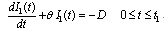
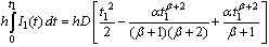
Considering the effect of demand and deterioration during [0,t₁] the inventory level at any instant of time during [0,t₁] can be described by the following differential equation

Now putting the value of θ in above equation we get,

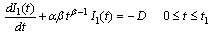(1)

Further the inventory level reaches zero at time t=t₁ Using this boundary condition we have. Again since α is very small, using series expansion and ignoring second and higher powers of α, from (1) we get,

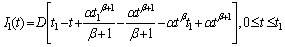(2)

Since inventory level reaches to zero at time t₁ and there after shortages occur. During the interval, the inventory level depends on demand and a fraction of the demand is backlogged. The state of inventory during can be represented by the differential equation,

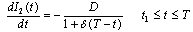(3)

Since inventory level reaches to zero at time, the boundary condition and the solution of the differential equation (3) is

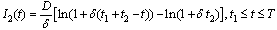(4)

Thus the maximum inventory will be

(5)

and the maximum backordered units will be

(6)

So, the order size Q during [0,T] will be

(7)

The following cost components need to be considered to calculate total cost per cycle:

i. Ordering cost per cycle is A

ii. Holding cost per cycle is

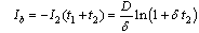
iii. Backorder cost per cycle

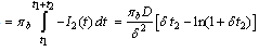iv. Cost of lost sales per cycle

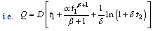
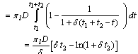v. Purchase cost per cycle

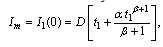
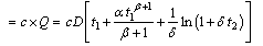Therefore, the total average cost per unit time is

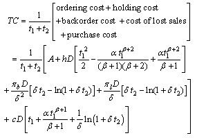(8)

The necessary conditions for minimizing the total average cost per unit will be

(9)

and

(10)

The pair of calculated from equations (9) and (10), subject to the condition

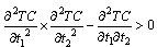will minimize TC.

Now we have

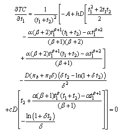(11)

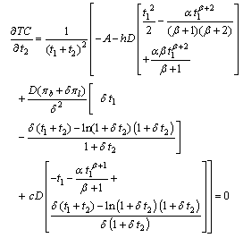(12)

The above set of parametric equations (11) and (12) can be solved for and using mathematica-5.1 software. Now we will consider a numerical example to illustrate and validate the proposed model in the following section.

5. Numerical Example

Example-1: Let an inventory system have the following parametric values in proper units.

[] =[200, 20, 0.7, 12, 10, 20, 2, 0.3, 0.2]. Using these values for the above model, we get optimum value of , putting the optimum values of and in equation (7) and (8) we get the optimum values of and minimum total average cost per unit time respectively.

6. Sensitivity Analysis

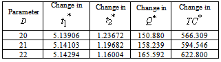
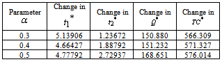
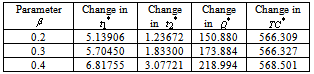
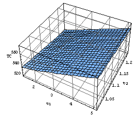
Now we will perform sensitivity analysis by increasing parameters and D , one at a time and keeping the remaining parameters at their original values. We will be using the values of the numerical example given in the previous section for performing the sensitivity analysis. The results are given in tabulated form in Table-1 to Table-4.

In table-1, it is observed that increase in demand parameter D results in increase in TC of an inventory system and also increase ordering quantity.

Table 1. Variation in demand D

Table 2. Variation in deterioration rate ‘α’

In table-2, it is observed that increase in deterioration rate ‘α’ results in increase TC of an inventory system and also increase ordering quantity.

Table 3. Variation in deterioration rate ‘β’

In table-3, it is observed that increase in deterioration rate ‘β’ results in increase TC of an inventory system and also increase ordering quantity.

Table 4. Variation in backlogging parameter ‘δ’

In table-4, it is observed that increase in backlogging parameter δ results in decrease in TC of an inventory system and decrease ordering quantity.

The results observed above can also be represented graphically in form of the following Figures.

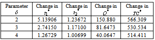
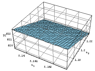Figure 1. Total cost TC versus t1 and t2 for table-1

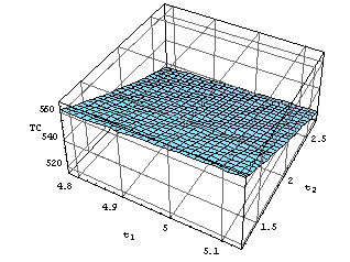Figure 2. Total cost TC versus t1 and t2 for table-2

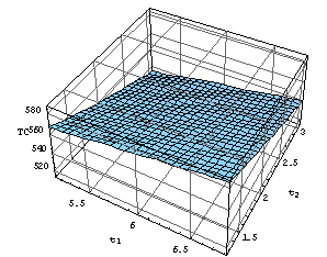Figure 3. Total cost TC versus t1 and t2 for table-3

Figure 4. Total cost TC versus t1 and t2 for table-4

7. Conclusions

In the present scenario of inventory system, large amount of capital is invested for purchase of inventory. It is important to consider deterioration in inventory decision making. In this paper a deterministic inventory model has been developed for Weibull deterioration. Shortages are allowed and are partially backlogged for this model. The unsatisfied demand is backlogged and is a function of time. The optimal order quantity has been derived by minimizing the total inventory cost. This will help in inventory decision making under similar condition. A numerical example and sensitivity analysis are presented to illustrate the proposed model. It is observed that increase in demand parameter or scale or shape parameters of deterioration function results in increase in total cost of an inventory system and also increase in ordering quantity. Further studies in this direction can be carried out incorporating more realistic assumption such as stochastic demand and finite replenishment rate.

ACKNOWLEDGEMENTS

We are highly indebted to the anonymous referees for their valuable suggestion and comments to improve upon the earlier version of this article to the present form.