1. Introduction

Healthcare both more efficient and patient centered. In the ambulatory setting this has frequently been interpreted as having patients spend more of their appointment time in direct interaction with the provider and less time waiting. Excessive wait time has been associated with lower patient satisfaction and compliance with treatment[8-11], patients leaving without completing their appointments[14], missed opportunities to provide preventive services[12], disgruntled staff[13], and reduced revenue to cost ratios. Underscoring the importance of reducing unnecessary patient waiting is the Joint Commission standard LD.3.15 requiring major health- care organizations to reduce unnecessary patient waiting as part of their certification program[15].

Crucial to minimizing wait times is understanding and controlling the consequences of patient scheduling. Not surprisingly, there is considerable interest in optimizing scheduling. The typical scheduling convention is to give patients an appointment at a specific time. Patients, however, commonly deviate from their scheduled appointment. Given the randomness of ‘timeliness,’ queues develop and providers find themselves either rushed to service the queue or idled as they wait for a patient to be “roomed”[6,7]. Clinical researchers have tried to address the queuing problem with ad hoc experiments using ‘open access’ or simulations – results are mixed[3,16].

Several authors have examined queue creation using discrete event simulation[1,4,5] while others have analyzed patient arrival patterns to identify the appropriate probability distribution for realization[1,15-19]. Most have recommended that offset times (i.e., deviation from scheduled appointment time) be sampled from normal distribution. Alexopoulos et al.[1] have suggested Johnson SU probability distribution. The consequences of using each of these different distribution families in modeling arrival patterns, developing discrete event simulations or in creating optimization schedules could be significant and warrants more study.

The normal distribution is a continuous probability distribution that often gives a good description of data that cluster symmetrically around the mean. The graph of the associated probability density function is bell-shaped, with a peak at the mean. In the Central Limit Theorem, the sum of a number of i.i.d (independent and identically distributed) random variables with finite means and variances approaches a normal distribution as the number of variables increases. The theorem will hold even if random variables are not i.i.d., although some constraints on the degree of dependence and the growth rate of moments still have to be imposed. Central Limit Theorem is an appropriate model for averaging observations.

We will show that normal distribution is seldom suitable for representing patient offset times. Johnson distribution SU[1], although providing an acceptable fit, is not the most stable fitted distribution.

Estimation of Distribution Function mainly contains three steps: choice of a model, finding the parameters, and analysis of error (e.g., checking that the model does not contradict observation). These steps are the core of a parametric estimation procedure to model the distribution. The choice of a family of distributions to model often depends on experience from studies of similar experiments or by analysis of data.

Before attempting to fit a probability distribution to a set of observed data, it is worth first considering the properties of the variable in question. The properties of the distribution or distributions chosen to be fitted to the data should match those of the variable being modeled. As an example, range of variable should match that of fitted distribution. Any interpretation of data requires subjective inputs, usually in the form of assumptions about the variable. The key assumption here is that observed data is randomly sampled from a probability distribution we are attempting to identify. It is assumed the observed data are both as reliable and representative as possible; anomalies in the data were checked and unreliable data points discarded. We also paid attention to possible biases that could be produced by method of data collection.

We are going to look at techniques to interpret observed data for a variable in order to derive a distribution that realistically models its true variability and our uncertainty about that true variability.

In this study, we will first find estimated parameters of statistical distributions that best fit patient offset times. Second, we will study the over-the-samples stability of the estimated parameters of the statistical distributions that best fit patient offset times and choose among such best fit distributions the one that exhibits the largest degree of stability in its estimated parameters. That is to say, if the entire body of data is a set S ofelements, , then a subsample of size is a proper subset of the set S (that is, ). Moreover, for the purpose of random sampling, the elements of the sub-sample are randomly chosen from the elements of the set S. If is sufficiently smaller than n, then from S one can draw many sub-samples, . Any suitable statistical distribution can be fitted to the data in these samples to obtain its estimated parameters. Obviously, there will be sampling variations in the estimated parameters. If the sample variations are within reasonable limits, estimated parameters are stable over the sub-samples.

We have considered numerous distributions such as Beta, Burr (4P), Cauchy, Chi-Squared (2P), Dagum (4P), Erlang (3P), Error, Error Function, Frechet (3P), Gamma (3P), Generalized Extreme Value, Generalized Gamma (4P), Generalized Logistic, Gumbel Min, Gumbel Max, Generalized Pareto, Hypersecant, Inv. Gaussian, Johnson-SU, Kumaraswamy, Laplace, Levy (2P), Log-Logistic(3P), Logistic, Normal, Pearson-5 (3P), Pearson-6 (4P), Pert, Rayleigh (2P), Weibull, and Wakeby. It is worth noting that all these distributions, except the Normal distribution, are either asymmetric or non-mesokurtic or both. We expect the best fit distributions to be both skewed and non-mesokurtic. The goodness-of-fit of the distributions is measured by three statistics pertaining to Kolmogorov-Smirnov (KS), Anderson-Darling (AD) and Chi-squared (CS) tests. In addition, three information criteria; SIC (Schwarz information criterion)[20], AICC (Akaike information criterion)[21-22], and HQIC (Hannan-Quinn information criterion)[23], are also used.

The remainder of this article is organized as follows: We briefly review some theoretical concepts in Section 2 to keep this article self-contained. Section 3 introduces the genesis and main features of the Generalized Logistic model and notes the model is leptokurtic and with skewness and kurtosis governed only by one parameter. This section also provides some results concerning the Maximum Likelihood (ML) and Method of Moments (MOM) estimates of the Generalized Logistic parameters and its quantiles. In Section 4, a simulation study is carried out in order to appraise the over-the-sample performance of different candidate distribution functions that best fit patient offset times data. Section 5 explains fitting second-order distributions to observed data points and reports the results of application of Generalized Logistic distribution to the available sampled data and error estimation using Generalized Bootstrap method.

2. Theoretical Review

2.1. Von Neumann’s test for independence

Von Neumann[24] proposed what is now known as the Von Neumann ratio:

where.

This can be approximated as:

, where is sample variance of the data.

If data are i.i.d., Von Neumann ratio distribution is very close to normal distribution. One can reject the hypothesis of independence at level when where is the of the standard distribution. The value is the user specified type I error (type I error is rejecting the null hypothesis when in fact it is valid). The p-value of this test is approximatelywhereis the CDF of standard normal distribution. The p-value of a test is the probability that a test statistics larger than the current one would be obtained if the hypothesized distribution were correct.

2.2. Parameter Estimation

The distribution parameters that make a distribution best fit the data can be determined in several ways, among them the method of maximum likelihood, moment matching, quantile matching, and least square[25]. The choice of estimators is governed by principles and criteria that provide objective basis for comparing the alternatives, among them sufficiency, completeness and ancillary. Assumeare the observed values of n i.i.d. random variables, each having a density function identical to .An estimator of is some function of the random variables and thus may be written as a notion that emphasizes this estimator is itself a random variable.

Various variable criteria have been proposed for an estimate to satisfy, among these are be unbiased, consistent and with low valiance of. It would also be desirable ifhas, either exactly or approximately, a normal distribution since well-known properties of normal distribution can then be used.

2.2.1. Maximum Likelihood Estimator

The Maximum Likelihood Estimator (MLE) method is fundamental in finding estimates of parametersin a statistical distribution model and is the most widely used. The theory of MLE estimates has deep consequences for many fields in statistics (see[26]). Statistical properties of the MLE are also useful, as will be later discussed. The Maximum Likelihood Method considersindependent observations and study the likelihood function defined as joint probability density for the observed dataset. The maximum likelihood estimator (MLE) of a parametric distribution are the values of parameters that maximize . Consider a probability distribution type defined by a parameter vector. The likelihood function of set of n data points could be generated from the distribution with probability density function as:

The MLE is then the value of that maximizes.

or equivalently

In a majority of cases, whenever the density function is well behaved

For some distribution types, the MLE calculation is a relatively simple algebraic problem; for others the differential equation is extremely complicated and is solved numerically. It is known that MLE has some asymptotic properties among them:.

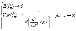One very important point is that MLE depends strongly on the parametric family chosen. Numerous studies examining the “robustness” of the MLE have identified how “wrong” a model can be when the incorrect distribution family is used. The best justification for the MLE is in its asymptotic properties, it turns out to be asymptotically optimal.

2.2.2. Moment Matching Estimator

The sample moments are functions of an i.i.d. sample whose probabilistic structure is determined a priori by the statistical model chosen. The probability distribution moments are often the best way to handle the unknown parameters. This relationship is exemplified by the raw moments below:

Given a random sample, thesample moment is The moment estimator of population parameters are obtained by matching the sample moments to the corresponding population moments and solving the resulting equations simultaneously.

2.2.3. The least square method

Let be random variables, not necessarily identically distributed, and set The least-squares method is estimating values, say such that the sum of square of error minimizes the loss function:

over. That is:

Least square method is not necessarily asymptotically efficient and can be quite sensitive to heavy trails (i.e., outliers/error contamination)

2.3 Fitting a second-order parametric distribution to observed data

The main issue in estimating the parameters of distribution from data is that uncertainty distributions of estimated parameters are usually linked together in some way. Historically it is assumed that parameter uncertainty distributions are normally distributed; however, this is not true for most cases.

To pursue fitting second-order distributions to observed data points, we need additional techniques for quantifying the uncertainty of distribution parameters. Among those techniques are bootstrap, Bayesian inference and some classical statistics methods. The parametric bootstrap technique is well suited, since one simply resamples from the MLE fitted distribution in the same size of the observed data. Data fitting using MLE again gives us random samples from the joint uncertainty distribution for the parameters.

2.3.1. Analysis of Estimation Error

The exact value of the estimation error is unknown-it is an uncertain value. The variability of the error can be studied using the following random variable,

the estimation error. For consistent estimators, tends to zero as n increases without bounds.

We can study the distribution of, which, for example, can be used to find intervals that, with high confidence, we can claim is in these intervals.

The ML estimators possess many good properties. For example, it can be shown (see[25] or, for a review,[26]) that ML method is a consistent estimator if satisfy certain regularity conditions, and be independent observation variables. The consistent estimators are defined as estimators that the error tends to zero as the number of observations n goes to infinity[27].

It is shown in[25] that if satisfies certain regularity conditions, ML estimators, behave asymptotically normal. Asymptotic normality means that for large n where, and

Estimation Error analysis can be performed numerically by parametric bootstrap method[28]. Bootstrap methods are most commonly used for complicated statistical problems, e.g. when the parameter is a large vector, or when an analytical approach is not possible.

For bootstrap methods, a computer program for Monte Carlo simulation is necessary. If the parameter, equivalently, the distribution is known, such a program can simulate independent samples, where N is some large integer. All these samples have the same random properties as our initial sample x and from each sample estimated are calculated

The error distribution can be approximated by means of the empirical distribution of, with increasing accuracy as N goes to infinity.

Let be the empirical distribution describing the variability of the sequence. (Note that the empirical distribution depends both on the number n of observations in our original data set and the number N of bootstrap simulations). Usually N is much larger than n since it is only limited by the computer time we wish to spend for the simulations. Finally, one can prove that, under suitable conditions, with,

Using the last result, if n is large we have an approximation of the error distribution.

The bootstrap quantiles defined by , are close to the quantiles .Thus an interval, which with (approximately) confidence, covers the unknown parameter is given by

2.4. Goodness–of-Fit Statistics

Many GOF (goodness-of-fit) statistics have been developed, but two are most commonly used. These are chi-square and Kolmogorov-Smirnoff (K-S) statistics. The Anderson-Darling statistic is a modification of K-S statistics. The lower the value of these statistics, the closer the distribution fits the data. GOF statistics do not provide a true measure of the probability that the data actually come from the fitted distribution. Instead, they provide a probability that random data generated from the fitted distribution would have produced a GOP as low as that calculated for the observed data. Analysis of the, K-S, and A-D statistics can provide confidence intervals proportional to the probability that fitted distribution could have produced the observed data.

Critical values are determined by the required confidence level-they are the values of the goodness-of-fit statistics that have a probability of being exceeded that is equal to the specified confidence level. Critical values of K-S and A-D statistics have been found by Monte Carlo simulation[29]. K-S and A-D statistics are designed to test whether a distribution of known parameters could have produced the observed data. If the parameters of the fitted distribution have been estimated from the data, they will produce conservative results. One way to circumvent this problem is to use a portion of data for estimation and remaining data for GOF test.

2.4.1. The chi-square () statistics

Chi-square () statistics measures how well the expected frequency of the fitted distribution having a CDF compares with the frequency of the observed data points. To conduct the most effective version of the test, we first divide the hypothesized distribution’s support into k”equiprobable” non-overlapping intervals; we identify valuessuch that, for where is the inverse CDF. The respective intervals are . We then compare the number of observation that fall in each interval; to the corresponding expected number; .The chi-square statistics is calculated:

,

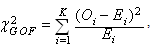where

Critical values for theare found from the distribution. The shape and range of the distribution are defined by the degree of freedom d, where, number of parameters that are estimated. We reject the null hypothesis that is the appropriate distribution, if where is the of chi-square distribution with d degree of freedom.

Since thestatistics sums of the square of all of the error, it can be disproportionately sensitive to any large errors. However, it is very dependent on the number intervals. For better results, n usually needs to be sufficiently large and k sufficiently small that It is recommended that the number of intervals to be chosen using Scott’s[30] formula.

2.4.2. Kolmogorov-Smirnoff (K-S) Statistic

Kolmogorov-Smirnoff (K-S) Statistics measures the vertical distance between CDF of the fitted distribution function and CDF of the observed data.

Assume data arising from a continuous distribution having a CDFNow let denote the order statistics based on the sample.The K-S statistics is defined as

,

where is known as K-S distance, n is the number of observed data points, for , where is the commutative rank of the data point, and is the distribution function of fitted distribution. It is well known Glivenko-Cantelli lemma[31] that, as the sample size n becomes large, the empirical CDF converges uniformly to for all x.

The K-S test quantifies both the maximum deviation of empirical CDF above or below the uniform line. The upper and lower empirical CDF are calculated as follows:

The K-S test rejects the hypothesized distribution when the test statistics

is larger than a tabulated quantile based on the sample size and the type I error.

The K-S statistic is generally more useful than statistic in that the data are assessed at all data points which avoids the problem of determining the number of intervals into which the data must be split. However, its value is only determined by the one largest discrepancy and takes no account for lack of fit across the remainder of distribution.

The vertical distance between the observed distribution and the fitted distribution at any point has a distribution with a mean of zero and a standard deviationgiven by binomial theory:

This indicates that the position of along the x axis is more likely to occur where is greatest, which generally is away from the low-probability tails. This insensitivity of K-S statistic to lack fit at the extremes of the distributions is corrected for in Anderson-Darling statistic.

2.4.3. Anderson-Darling (A-D) statistic

The A-D statistic is defined as:

where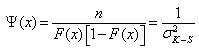

.

n is the number of observed data points, is the CDF of fitted distribution, is the density function of fitted distribution, , for cumulative rank of the observed data point and is the number of non-overlapping intervals.

The Andeson-Darling statistic is an improved version of Kolmogorov-Smirnoff statistic. compensates for the variance of the vertical deviation distance between sample distribution and fitted distribution ().weights the distance by the probability that a value be generated at that x value. The vertical distances are integrated over all values of x to make maximum use of observed data (the K-S static only look at the maximum deviation distance).

The A-D statistic

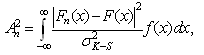is therefore generally a more useful measure of goodness of fit than the K-S, especially where it is important to place equal emphasis on fitting a distribution at the tails as well as at main body. Nonetheless, it still has the same problem as K-S statistic i.e., the fitted distribution should, in theory, not be estimated from the data.

2.4.4. A better Goodness-of-Fit Measure

For reasons explained above, the chi-square, Kolmogorov-Smirnoff and Anderson-Darling goodness-of-fit statistics are technically all inappropriate as a method of comparing fits of distributions to data. They are also limited to having precise observations and cannot incorporate censored, truncated or binned data. Realistically, most of the time we are fitting a continuous distribution to a set of precise data observations and, under these circumstances, Anderson-Darling proves adequate. However, for important work we should instead consider using statistical measure of fit called information criteria. Let n be the number of observations, s number of parameters to be estimated and be the maximized value of likelihood function.

SIC (Schwarz information criterion, aka Bayesian information criterion, BIC)[20]

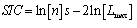AICC (Akaike information criterion)[21-22]

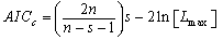HQIC (Hannan-Quinn information criterion)[23]

The aim is to find the model with the lowest value of the selected information criterion. The term appearing in each formula is an estimate of the deviance model fit. The coefficients of in the first part of each formula, shows the degree by which the number of model parameters is being penalized. For the SIC[20] is the strictest in penalizing loss of degree of freedom by having more parameters in the fitted model. For AICC ([21-22] is the least strict of the three, and HQIC[23] is in between.

3. The Model

A theoretical representation of patient offset times distribution have traditionally relied on two-parameter cumulative density functions because these are relatively easy to estimate. However, the two-parameter models cannot deal with the existence of leptokurtic and skewness without the introduction of assumptions that limit their goodness-of-fit, Instead, Alexopoulos et al.[1] offered Johnson SU which treats skewness nicely but here we will show that it lacks the stability properties of Generalized Logistic distribution.

3.1. Genesis and Properties of the Hosking Generalized Logistic Distribution

The generalized logistic distributions are very useful classes of density functions as they possess a wide range of indices of skewness and kurtosis. Therefore, an important application of the generalized logistic (GL) distribution is its use in studying robustness of estimators and tests.

The GL distribution is a generalization of the two- parameter logistic distribution and is also a special case of the kappa distribution[32]. This generalization of the logistic distribution differs from other distributions defined in the literature. The cumulative distribution function and the probability density function of the GL distribution are defined respectively[2].

Let X be a positive continuous random variable that belongs to the family of Hosking GL distribution with three parameters. Its CDF and density distribution is:

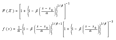where is the location parameter, is the scale parameter, and is the shape parameter. The range of possible values for the GL distribution is given by

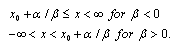Note that as a special case, if then the GL distribution is reduced to the two-parameter logistic distribution. Additional generalizations of the logistic distribution are discussed[33].

The mean, variance, and Fisher’s coefficient of are[33]

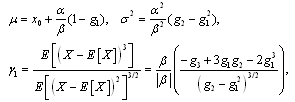where is the gamma function, and exists only if Since is location and scale invariant the skewness of the distribution depends only on parameter. A random variable X with generalized logistic distribution has a variance depending on the parametersand .The quantile estimator of the GL distribution can be obtained by substituting and solving for x

where are the parameter estimators, and T is the return period[33].

Method of moments (MOM)

The skewness coefficient of the GL distribution is only a function of the shape parameter. Then can be approximated as follows[34]

A more precise estimate of the shape parameter can be obtained using a numerical approximation. Thethat minimizes[33]

is an approximation for the shape parameter. Once the she parameter is known, and can be obtained as follows:

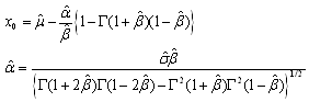Method of maximum likelihood (ML)

Consider a sample of size n of independent positive random variables. Let the log-likelihood function of the GL distribution is given by[33]

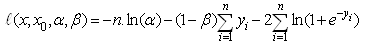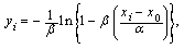wheren is the sample size, and represents the natural logarithm. The MLEs are obtained from the maximization of as the solution of the following likelihood equations or score functions:

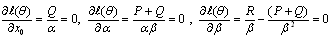where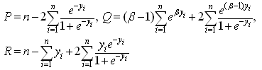

The system does not admit any explicit solution; therefore the ML estimatescan be obtained only by means of numerical procedures.

4. Best Fit Parameter Analysis

4.1. Data collection

A total of 738 patient observations were obtained from a variety of ambulatory care clinics as part of ongoing workflow data collection efforts. These observations were collected using a workflow data acquisition tool described in Fontanesi et al.[8]. This tool, the Observational Checklist of Patient Encounters (OCPE), includes data fields to record individual patient scheduled appointment times and actual observed arrival times.

4.2. Data Analysis

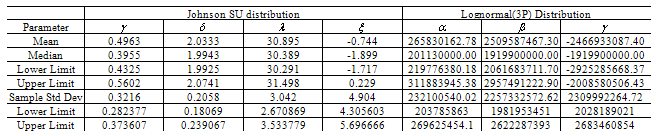
Three distributions emerge as best fit based on GOF tests and information criteria: Generalized Logistic, Johnson SU and Log-Logistic. In the majority of cases, either Generalized Logistic or Log-Logistic does better than Johnson SU on the criterion of KS or AD test. However, on CS tests, Johnson SU is emerges stronger than on KS or AD test. It may be noted that AD weights the fit more to the tails and CS weights the overall fit more. On information criteria test, again GL and Log-Logistic performed better than Johnson SU. This simply could be explained that information criteria penalizes for larger number of parameters (GL and Log-Logistic are 3 parameter distributions and Johnson is 4 parameter).

Algebraic form of the pdf of Generalized Logistic, Log-Logistic, and Johnson SU distributions are given as

i) Generalized Logistic Distribution

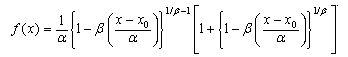
Where respectively are; continuous location parameter, scale parameter, and shape parameter.

ii) Log-Logistic (3P) Distribution

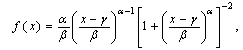where respectively are; continuous location parameter, scale parameter, and shape parameter.

Johnson SU Distribution

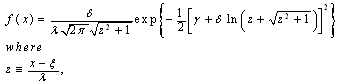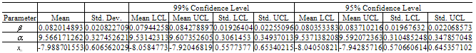
and are respectively; continues location, scale (), and shape () parameters.

The illustrative fits of Generalized Logistic, Johnson SU, and Log-Logistics distributions to sample data are presented in Fig.-1.

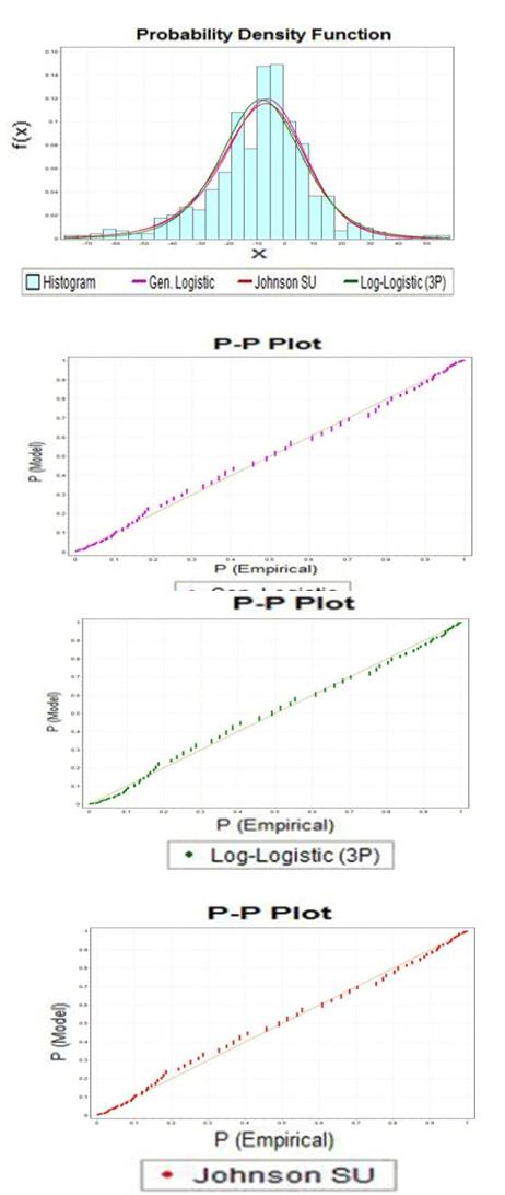Figure 1. Generalized Logistic, Johnson SU, and Log-Logistics distributions fit to sample data

Table 2.1. Measures of Central Tendency and Dispersion of Parameters of Generalized Logistic Distributions over Sub-samples (Confidence level %95, Sample Size 100)

Table 2.2. Measures of Central Tendency and Dispersion of Parameters of Johnson SU and Log-Logistic (3P) Distributions over Sub-samples (Confidence level %95, Sample Size 100)

4.3. Over-the-Samples Stability of the Estimated Parameters

Of the statistical distributions considered, the one that exhibits the largest degree of stability in its estimated parameters will be selected as the best fit best to patient offset times. For this analysis subsets of data each of length have been drawn randomly from a 738 points main sample data set. Estimated parameters, are tabulated in Tables 1.1, 1.2. Measures of central tendency and dispersion of the estimated parameters are presented in tables 2.1 and 2.2. The two measures of central tendency (median and mean) for all the parameters indicate their distributions are almost symmetrical and standard deviations are much smaller with respect to means[35].

It becomes readily apparent that the estimated parameters of the Generalized Logistic distribution exhibit better over-the-samples stability than the other two distributions.

5. Fitting Second-Order Distributions to Observed Data Points: the Generalized Bootstrap (GB) Analysis

In order to calculate uncertainty of distribution parameters[36] we will use the method of Generalized Bootstrap. The essence of the Generalized Bootstrap (GB) Method is to fit a distribution to the available data and then take samples from the fitted distribution (Bootstrap Method BM generally works with samples from the data). This method has been shown to perform better than the BM when the number of data points is not very large and do as well as the BM when the number of data points is large. Sun and Muller[37] have an excellent exposition with real-data examples.

Suppose that we are interested in some function of the distribution, and is unknown. However, we have a random sample, from, and we want to estimate.The Generalized Bootstrap (GB) approaches the problem as follows[38]:

Suppose that one would typically estimate by. Then, instead, proceed as follows: First, estimate . Second, independently generate N random samples of n from, and estimate for each sample. Third, use the sample to estimate. For example, one may calculate[37]

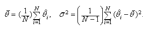which give the sample mean and sample variance, respectively, of the GB estimators .Then, assuming approximate normality, we have

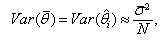and an approximateconfidence interval for based on standard method is

A widely used alternative to standard method is "percentlie method," which uses the upper and lowerpercentiles of the GB sample estimators as the confidence interval. Specifically, the percentlie method proceeds as follows: Place the N estimates in increasing numerical order, obtaining

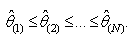The percentile methods’ (approximate) confidence interval foris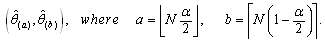

Sun and Muller-Schwarze[36] compared the performance of bootstrap method and generalized bootstrap and concluded that GB is more consistent in parameter estimation than BM. Asymptotic properties of GB have been shown by[28].

In this part of analysis we will independently generate random samples of length from a GL distribution

Table 3.2. Generalized Bootstrap Analysis of 517 sets of data of length 738

, and estimated for each sample. Estimated values of parameters, are shown in Table 3.1. The calculated values of mean, standard deviation and their lower and higher limits for different confidence intervals are presented in table 3.2 and 3.3.

Figure 2. Uncertainty in parameters of the Generalized Logistic distribution fitted to patient’s offset times

6. Conclusions

Service industries, to include health care, have shown value is co-produced, perishable and time-sensitive.

In the health care clinic setting, surveys reveal the greater the amount of time a patient spends with a provider relative to total clinic time, the greater the potential degree of value co-production. To apply the science of health care quality to primary, practical application, one of our research groups’ targets is the consequences of queues and crowding in the clinic setting and, concomitantly, in developing tools that may be utilized to create appointment schedules and allocate staff in order to provide a maximum number of patients the highest quality service.

Several interesting findings arose from our analysis of patient waiting times in the clinic venue. First, patient offset times in scheduled visits do not follow a normal distribution; indeed the distribution is not even symmetric. Second, three distributions, Generalized Logistic, Johnson SU and Log-Logistic, nicely fit the observed data points. Third, Generalized Logistic showed a high degree of stability in over-the-sample stability analysis. Due to these outcomes, we recommend anyone engaged with modeling activitiesinvolving assumptions about patient arrival patterns be cautious when choosing the distribution of random variables.

To affect practical change, an important remaining task is to examine the real-life consequences of applying an ill-fitting distribution[1]. What is the implication, for example, in using a slightly incorrect patient offset time distribution in developing patient scheduling schemas? We predict failure to properly characterize patient’s offset times is likely to result in unnecessary congestion and wait times as patient queue’s emerge over the day[39, 40]. What are the broader implications to the quality of health care in using correct or ill-fitting distribution assumptions in scheduling patients? Thus, ongoing work includes optimal scheduling policies for patients and staff, improvement of medical practices to insure better levels of treatment, and the development of clinic policies in cases of unusual levels of patient demand. Provided that adequate and reliable data are obtained, one of the most obvious ways to study these problems is through the use of computer simulation techniques.