1. Introduction

The classical inventory models considered the case where the replenishment is done instantaneously i.e. at an infinite rate. Keeping this situation in mind a number of researchers produced a number of inventory models with replenishment at an infinite rate. Covert and Philip (1973) formulated an EOQ model in which the rate of deterioration of inventory involves two-parameter Weibull distribution, demand rate is a constant and the instantaneous replenishment occurs without shortage of inventory. Wee (1997) discussed a replenishment policy for items with varying rate of deterioration and demand being dependent on the price level of item. Zhao and Zheng (2000) deduced the optimum value of price which is dynamic in nature for perishable assets by assuming that the nature of demand is heterogeneous. Ghosh and Chaudhuri (2004) developed an inventory model for a deteriorating item having an instantaneous supply, a quadratic time-varying demand and shortages in inventory. A two-parameter Weibull distribution is taken to represent the time to deterioration. Balkhi and Bakry (2009) considered a dynamic inventory model with deteriorating items in which each of the production, the demand and the deterioration rates, as well as all cost parameters are assumed to be general functions of time. Das and Reza (2009) establish an economic order quantity (EOQ) model for deteriorating itemsduring phases of production , deterioration and backlogging. Begum et al. (2010) investigated inventory-production system where the deteriorating items follow two parameters Weibull deterioration. They developed the order level inventory models for deteriorating items with quadratic demand. Li et al. (2010) reviewed the recent studies in deteriorating items inventory management research fields. He proposed some key factors which should be considered in the deteriorating inventory studies. Kalam et al. (2010) considered the production inventory problem in which the deterioration is Weibull distribution; production and demand are quadratic function of time. The solution of the model is discussed for finite time horizon.

Kang and Kim (1983) studied on the price of the deteriorating inventory, since is most important factor of demand as well as production so, production level at the firm decided on the basis of price. In order to quantify it, Baker and Urban (1988) established an economic order quantity model for deterministic inventory system with power form inventory level dependent demand pattern. Datta and Pal (1988) dealt with a power demand pattern inventory model with variable rate of deterioration. Both deterministic and probabilistic demands have been considered.

Mandal and Phaujdar (1989) developed an economics production quantity model for deteriorating items with constant production rate in which consumption rate depends on stock linearly. It assumed that the more consumption takes place at more stock. Later on, Datta and Pal (1990) established an EOQ model in which the demand rate is a power function of the on-hand inventory displayed until down to a certain stock level, at which the demand rate becomes a constant. Pal et al. (1993) studied a deterministic inventory model for deteriorating items and the demand of item being stock dependent. Giri and Choudhury (1998) determined economic order quantity of perishable inventory with stock dependent demand rate and nonlinear holding cost. Kobbacy and Liang (1999) concerned with the development of an intelligent inventory management system which aims at bridging the substantial gap between the theory and the practice of inventory management. The models incorporated cover deterministic demand models including: constant, quasi-constant, trended and seasonal demand as well as stochastic demand models. Mishra and Singh (2000) presented the inventory models for damageable multi items and also focused on the consumption cost where demand depends on the available stock. Reddy and Sarma (2001) presented a periodic review inventory problem assuming that demand is stock dependent. Datta and Paul (2001) discussed an inventory system in which demand is stock dependent and more sensitive in the sense of price of item. Sana and Chaudhuri (2003) developed an inventory model of a volume flexible manufacturing system for a deteriorating item taking a stock -dependent demand rate. Demand rate remains stock-dependent for an initial period after which a uniform demand rate follows as the stock comes down to a certain level. The unit production cost is taken to be a function of the finite production rate. Ouyang et al. (2005) proposed an EOQ inventory mathematical model for deteriorating items with exponentially decreasing demand.

Berman and Perry (2006) presented a model in which demand rate is the function of inventory level and it is a piecewise constant function and a family of exponential functions. The demand functions and holding cost functions considered as quite general. Jain et al. (2007) presented an economic production quantity (EPQ) model for deteriorating items with stock-dependent demand and shortages. They assumed that a constant fraction of the on-hand inventory deteriorates and demand rate depends upon the amount of the stock level. Zhou and Shi (2008) developed a deterministic inventory model for deteriorating items with stock- dependent demand. Ghosh and Chakrabarty (2009) considered an order-level inventory model with two levels of storage for deteriorating items assuming that the demand is time- dependent. Panda et al. (2009) considered a single item economic order quantity model in which the demand is stock dependent. After a certain time the product starts to deteriorate and due to visualization effect and other aspects of deterioration the demand becomes constant. Singh et al. (2009) developed an inventory model in which demand follows power pattern. When fresh and new items arrive in stock they begin to decay after a fixed time interval. Skouri and Konstantaras (2009) considered an order level inventory model for seasonable and fashionable products subject to a period of increasing demand followed by a period of level demand and then by a period of decreasing demand rate (three branches ramp type demand rate). The product deteriorates with a time dependent, namely, Weibull deterioration rate. Valliathal and Uthayakumar (2009) studied a deterministic inventory model for deteriorating items. They considered the combined stock and time varying demand to make the theory more applicable in practice. Patra et al. (2010) developed a deterministic inventory model when the deterioration rate is time proportional. Ghare and Schrader (1963) developed an inventory model for an item with an exponentially decaying inventory, constant demand and finally obtained economic order quantity for the model. Further, Philip (1974) extended the EOQ model by considering the deterioration rate as a variable which follows three-parameter Weibull distribution. Misra (1975) established the optimal production lot size model for deteriorating items with constant demand and varying deterioration as well as constant rate (exponential case) deterioration. He used a two-parameter Weibull distribution to fit the deterioration rate during the production of items and suggested a numerical method for varying rate of deterioration. Shah and Jaiswal (1977) considered an order-level of inventory for the system in which the rate of deterioration is constant (uniform). Cohen (1977) established the joint pricing and ordering policy for exponentially decaying inventory with known demand. Gupta and Vrat (1986) considered an inventory model of stock-dependent consumption rate. Padmanabhan and Vrat (1995) studied EOQ models for perishable items under stock dependent selling rate. Wu et al. (1999) considered an EOQ model in which inventory is depleted not only by demand, but also by deterioration at a Weibull distributed rate, assumed the demand rate with a ramp type function of time. Chen and Lin (2002) focused on optimal replenishment inventory items and assumed that the deterioration is distributed normally. Mishra et al. (2002) have discussed an inventory models for damageable items with two-level storage facility and occurrence of breakdown of machines.

Dye (2004) proposed an EOQ model for perishable Items with Weibull distributed deterioration. He assumed that the demand rate is a power-form function of time. Sana and Chaudhuri (2004) developed a stock-review inventory model for perishable items with uniform replenishment rate and stock-dependent demand. The deterioration function per unit time is a quadratic function of time. The associative cost function is optimized due to the limitation of storage capacity. Deng (2005) considered inventory models with ramp type demand for items with Weibull deterioration. Mishra and Mishra (2008) determined optimum quantity and the price of deteriorating inventory item under perfect competition using marginal revenue and marginal cost approach for different level of stock based demand because it attracts more customers to buy more. In this model the effect of number of selling point in the market on the demand is also discussed. Roy (2008) developed a deterministic inventory model when the deterioration rate is time proportional. Demand rate is a function of selling price and holding cost is time dependent. He considered both the cases shortage and no-shortage in inventory. Shah and Acharya (2008) formulated an order-level lot-size inventory model for a time – dependent deterioration and exponentially declining demand. Singh et al. (2009) considered an inventory problem for a deteriorating item having two separate warehouses, one of finite dimension and the other of infinite dimension. Deterioration rates of items in the two warehouses may be different, which is time dependent and the demand rate of items is linear with time. Arya et al. (2009) presented an optimization framework to derive optimal replenishment policy for perishable items with stock dependent demand rate. The demand rate is assumed to be a function of current level inventory and the inventory deteriorates per unit time with variable deterioration rate. These two parameter and third-parameter Weibull distribution functions are considered as variable deterioration rate.

Tripathy and Mishra (2010) dealt with development of an inventory model when the deterioration rate follows Weibull two parameter distributions, demand rate is a function of selling price and holding cost is time dependent. With shortage and without shortage both cases have been taken care of in developing the inventory models. Tripathy et al. (2010) developed an order level inventory system for time dependent linearly deteriorating items with decreasing demand rate, assuming that the production rate and the demand rate are time dependent. Two EOQ models for without shortage case and with shortage case have been developed. Kundu and Chakrabarti (2010) considered economic order quantities under conditions of price dependence of demand. In first model, the rate of deterioration is taken to be time-proportional and a power law form of the price dependence of demand is considered. In second model, the rate of deterioration taken to be time-proportional and the time to deterioration is assumed to follow a two-parameter Weibull distribution. A power law form of the price-dependence of demand is considered. They assumed that the time where the inventory depletes to zero is a random point of time.

Sana and Chaudhuri (2004) attempted the model analytically with power order deterioration but they made no attempt to solve the model numerically because of mathematical complexity of the model. As a result, no sensitivity analysis leading to economic feasibility of the model was attempted to study the variation of total optimal average cost of the model with the variation of various important parameters involved in the model. With this in mind in this paper, a computational algorithm has been developed to find the numerical solution of the model having cubic deterioration by solving the complex problem of non-linearity by using a set of techniques of N-R and Taylor’s series to compute the total optimal average cost of the system as an important performance measure of the model. All the computations regarding the performance measures are carried out with the help of computing algorithm and its implementation in the C++ language. An exhaustive numerical demonstration and sensitivity analysis have been presented with the help of computing algorithm to exhibit the use of the model. Advantage of the present investigation of the problem lies in the fact that an important performance measure of total optimum average cost of the system is computed to gain the better insight for planning and controlling the production of the inventory. The provision of cubic deterioration is another useful novelty of the model to assess the reliability of the deterioration of inventory with respect to volatile items.

The whole paper has been organized in various important sections which include introduction, fundamental assumptions and notations, model development and its cost analysis, computing algorithm, numerical demonstration and sensitivity analysis and conclusion.

2. Fundamental Assumptions and Notations

We have used the following assumptions and notations for the model formulation.

Assumptions

i. Demand of perishable items depends upon on hand inventory. The demand function is taken to be a power form function of inventory level at any time as, , , where and are scale and shape parameters. The pictorial representation of demand function is shown in the following figure:

Figure 3.1. Power form demand rate-time relationship

ii. Replenishment rate is infinite (instantaneous) but replenishment size is finite.

iii. Replenishment rate is uniform.

iv. Lead-time is zero.

v. Inventory model is considered for a single perishable product.

vi. A variable fraction of the on-hand inventory deteriorates per unit of time and is a cubic function of time. Here where are real numbers, So that

a)

b)

c)

where a = initial deterioration, b = initial rate of change of deterioration, c = acceleration of deterioration and d = rate of change of acceleration of deterioration. The items undergoes decay at θ(t)I(t) at any time t. The intensity of deterioration is very low during the early stage of inventory because t is small. However, the intensity increases with time rapidly as it is a cubic function of time. The pictorial representation of deterioration function is shown in the following figure:

Figure 3.2. Deterioration-time relationship

vii. Storage capacity is limited.

viii. Shortages are not allowed.

ix. All ordered units arrive new and fresh, that is, their age equals zero.

x. The time-horizon is infinite.

xi. Holding cost per unit per unit time and set-up cost per inventory cycle both are constant.

xii. Procurement cost (i.e. costs to acquire inventory from various manufacturing centers or units) per unit item is also constant.

Notations

I(t)=On hand inventory at time t.

I1=Starting and ending inventory level.

I2=Pick of the inventory level.

R=Finite replenishment rate.

Cs=Set up cost per cycle.

Ch=Holding cost per unit per unit time.

Cp=Procurement cost per unit item.

t₁=Pick off time of the inventory level.

T=The length of a cycle.

TAC=Total average cost for a replenishment cycle.

3. Model Development & Cost Analysis

The inventory system developed is depicted by the following figure:

Figure 2.3. Inventory level-time relationship

In this model, the inventory cycle time consists of two segments [0, t1] and [t1, T]. Uniform replenishment rate starts with inventory I1 and continues upto time t = t1. The inventory piles up during [0, t1], after meeting demands in the market. The inventory level at time t = t1 is I2. The storage space is limited here. It can store maximum (Ix) units. Again, the inventory level gradually reaches to I1 at time t = T. The instantaneous states of the inventory level at any timeare governed by the following system of differential equations:

(3.1)

(3.2)

Without loss of generality, we prefer to work,We solve the above equations by approximation using Taylor’s series expansion. Then eqn (3.1) reduces to so that

Applying initial condition at t = 0, viz

We get

Neglecting fifth and other higher order derivatives from the expansion of I(t), we have

(3.3)

Similarly, applying initial condition at t = t1 from eqn (3.2), we have

(3.4)

where

The total inventory in the cycle

(3.5)

Total cost invested during each inventory cycle is given by

Therefore, the total average cost is

(3.6)

Now we optimize

The optimal value of for the minimum total average cost is the solution of the non-linear equation in i.e. provided that this obtained value of satisfies the condition, where T* is the optimal value of T.

The above constrained optimization problem can be solved using any iterative numerical method when the values of the parameters are prescribed. Here, this objective is fulfilled by developing computing algorithm and using N-R method which returns us optimal value of T and total optimal average cost (TOAC) of the system.

4. Computing Algorithm

The following computing algorithm is developed to find out the optimal cycle time and total optimal average cost of the inventory system.

Step (i): Begin

Step (ii): Data input

Step (iii): Enter D

Step (iv): Enter Ch, Cs and Cp

Step (v): Enter deterioration rate

Step (vi): Enter initial guess of cycle time

Step (vii): Define function

Step (viii): Do

Step (ix): Compute function

Step (x): Compute function derivative

Step (xi): Compute

Step (xii): Compute diff. (Tn-To)

Step (xiii): Assign To=Tn

Step (xiv): While

Step (xv): Abs(diff)<0.0001 & diff. 0.

Step (xvi): Data output fn

Step (xvii): Data output fnd

Step (xviii): Data output Tn

Step (xix): Define total average cost function (tacf)

Step (xx): Enter Tn

Step (xxi): Compute tacf

Step (xxii): Data output tacf

Step (xxiii): End

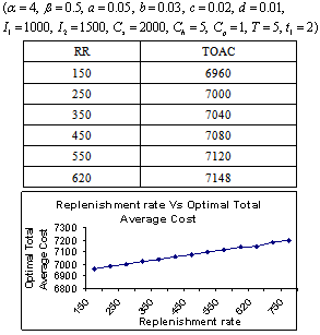
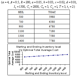
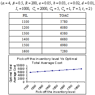
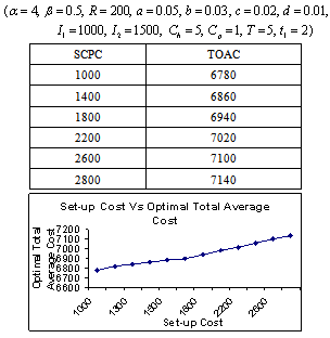
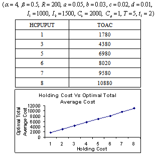
5. Numerical Demonstration & Sensitivity Analysis

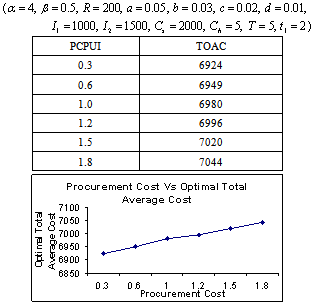
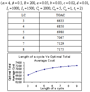
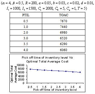
The following tables are the output of the computing algorithm implemented in C++.

Table and Graph 5.1. Replenishment rate (RR) Vs. TOAC

Table and Graph 5.2. Starting and ending inventory level (SEIL) Vs. TOAC

Table and Graph 5.3. Pick-off inventory level (PIL) Vs. TOAC

Table and Graph 5.4. Set up cost per cycle SCPC Vs TOAC

Table and Graph 5.5. Holding cost per unit per unit time HCPUPUT Vs TOAC

Table and Graph 5.6. Procurement cost per unit item PCPUI Vs TOAC

Table and Graph 5.7. Length of a cycle LC Vs TOAC

Table and Graph 5.8. Pick-off time of inventory level PTIL Vs TOAC

The aim of the sensitivity analysis is to demonstrate the variability of the model based on the simulations or the hypothetical data-input. In this paper, we prefer the hypothetical data-input to run the search program of the system. It is the process of varying model parameters over a reasonable range and observing the relative changes in the model response. Remarkable are the observed changes in the total optimal average cost of the inventory model under consideration. We wrote a program in C++ to compute the total optimal average cost of the inventory model under consideration. In sensitivity analysis, variational effect of parameters on the total optimal average cost is presented. The following observations have been drawn from the model under consideration.

In table and graph (5.1), we observe that as replenishment rate increases, the total optimal average cost of the inventory cycle increases. Numerically, an increase of 17% in the replenishment rate of the inventory cycle amounts to increase of about 0.29% in total optimal average cost of the inventory cycle. It indicates that as replenishment rate of the inventory cycle increases, the system will be more economically feasible. Here is a positive correlation between replenishment rate and the total optimal average cost.

In table and graph (5.2), we see that as starting and ending inventory level increases, the total optimal average cost of the inventory cycle increases. In fact, about 20% increase in the starting and ending inventory level of the inventory cycle amounts to approx. 3.35% in total optimal average cost of the inventory cycle. Thus, we observe that changes in the total optimal average cost of the inventory cycle with respect to starting and ending inventory level is very slow. This also shows a positive correlation between starting and ending inventory level and the total optimal average cost.

In table and graph (5.3), we find that as pick of the inventory level increases, the total optimal average cost of the inventory cycle increases. Moreover, an increase of 9.1% in the pick of the inventory level of the inventory cycle amounts to increase of about 5.19% in total optimal average cost of the inventory cycle. Thus, the changes in the total optimal average cost of the inventory cycle with respect to pick of the inventory level are almost same. Here is a positive correlation between starting and ending inventory level and the total optimal average cost. This is in the complete agreement with the basic idea that the inventory level is directly proportional to the total optimal average cost of the inventory cycle in nature.

In table and graph (5.4), we find that as Set up cost per cycle increases, total optimal average cost of the inventory cycle increases. Further, an increase of 20 % in set up cost per cycle creates approx. 0.006 % increase in the total optimal average cost of the inventory cycle. There exists a positive correlation between set up cost per cycle and the total optimal average cost of the inventory cycle.

In table and graph (5.5), we see that as holding cost per unit per unit time of the inventory cycle increases, the total optimal average cost of the inventory cycle increases. Thus, a positive correlation is found between them. Moreover, 33.3% increase in holding cost per unit per unit time of the inventory cycle amounts to increase of about 29.68% in the total optimal average cost of the inventory cycle. Thus, almost same changes are observed in holding cost per unit per unit time of the inventory cycle with respect to the optimal total Average Cost of the inventory cycle.

In table and graph (5.6), we observe that as Procurement cost per unit item in the inventory cycle increases, the optimal Total Average Cost show an increasing trend. Actually, an increase of 20% in procurement cost per unit item in the inventory causes about 0.23 % increase in the optimal Total Average Cost of the inventory cycle. This shows a positive correlation between them.

From table and graph (3.7), it is clear that when length of an inventory cycle increases, the optimal total average cost show an increasing trend. Actually, an increase of 25% in length of an inventory cycle causes about 0.44 % increase in the optimal total average cost of the inventory cycle. This also shows a positive correlation between them.

From table and graph (5.8), it is clear that when pick off time of the inventory level increases, the optimal total Average Cost show a decreasing trend. Actually, an increase of 25% in pick off time of the inventory level causes about 3.3 % decrease in the optimal total average cost of the inventory cycle which shows a negative correlation between them.

6. Conclusions

It is a real fact that a large pile of goods motivated the customer to buy more. So the demand rate should be a function of the stock-level. In the literature, deterioration rate is considered as constant, linear, quadratic function of time and Weibull distribution. But we have considered the deterioration is a cubic function of time. Because, when deterioration starts then it is accelerated with time. This situation happens in case of fast deteriorating items such as meat, vegetables, fruits, dairy and allied products (milk, curd cheese, yoghurt, and Khoya etc), bread, sweets, food, and high nitrogen containing chips, pharmaceuticals, blood and radioactive chemicals. Shortages are not allowed.

As in the constructed model, the considered environment does not fit to any specific system but captures some common characteristics of that environment; the model developed provides the best possible solution subject to the model constraints. Various observations laid down (tables 5.1- 5.8) for the model to see the adaptability of the proposed model. The objective of our model is to determine the total optimal average variable inventory cost at optimal inventory-level, which is the sum of set-up costs, holding costs and procurement costs of inventory items.

ACKNOWLEDGEMENTS

The authors are highly thankful to the editor for improving the paper in the present form.