Darcy Warms1, Aarya Satardekar1, Anusha Parajuli1, Rishil Shah2, Spuritha Bhandaru1, Namit Choudhari3, Benjamin G. Jacob1
1Samuel P. Bell III College of Public Health, University of South Florida, Tampa, FL, USA
2Bellini College of Artificial Intelligence, Cybersecurity and Computing, University of South Florida, Tampa, FL, USA
3School of Geosciences, University of South Florida, Tampa, FL, USA
Correspondence to: Darcy Warms, Samuel P. Bell III College of Public Health, University of South Florida, Tampa, FL, USA.
| Email: |  |
Copyright © 2026 The Author(s). Published by Scientific & Academic Publishing.
This work is licensed under the Creative Commons Attribution International License (CC BY).
http://creativecommons.org/licenses/by/4.0/

Abstract
This study advances a mathematically rigorous, spatially explicit framework for identifying uterine cancer (UC) vulnerability through the detection of aggregation and non-aggregation-oriented hot and cold spots at the Zip Code Tabulation Area (ZCTA) level in Hillsborough County, Florida. Leveraging a semi-parametric eigen-spatial filtering (ESF) approach, the model integrates Poisson and negative binomial generalized linear formulations with eigenvector-derived spatial autocorrelation structures to address violations of independence and overdispersion inherent in epidemiological count data. Synthetic proxy variables representing socioeconomic, sociodemographic, racial, and healthcare access disparities were constructed to approximate latent vulnerability in the absence of complete individual-level data, thereby preserving privacy while enabling population-level inference. Spatial dependence was operationalized through contiguity-based weight matrices and decomposed via eigen-analysis, allowing the incorporation of orthogonal spatial basis functions into regression estimation to mitigate residual autocorrelation bias. Model optimization employed iterative selection of eigenvectors and smoothing parameters using information criteria and cross-validation to balance parsimony and explanatory power. Moran’s I statistics and permutation-based inference were utilized to evaluate spatial clustering and classify statistically significant high-risk and low-risk ZCTA regions. Results indicate that key predictors-including racial composition, median household income, and ethnicity-exhibit strong associations with UC vulnerability, reinforcing the role of structurally embedded inequities in shaping geographically patterned health outcomes. The resulting spatial risk surfaces provide actionable intelligence for precision public health interventions, including targeted screening, early diagnostic engagement, and geographically tailored social messaging strategies. This framework demonstrates the utility of integrating stochastic processes, spatial statistics, and covariate-informed modeling to enhance inferential validity and support scalable, policy-relevant cancer control initiatives.
Keywords:
Spatial data mining, Geospatial machine learning, Eigenvector decomposition, Spatial filtering algorithms, Graph-based modeling, Poisson regression
Cite this paper: Darcy Warms, Aarya Satardekar, Anusha Parajuli, Rishil Shah, Spuritha Bhandaru, Namit Choudhari, Benjamin G. Jacob, Moran's Eigen-Spatial Analytic Methods for Mapping Hot and Cold Spots of Uterine Cancer in Hillsborough County, Florida, American Journal of Mathematics and Statistics, Vol. 15 No. 1, 2026, pp. 10-20. doi: 10.5923/j.ajms.20261501.03.
1. Introduction
Uterine cancer, including endometrial carcinoma and other uterine neoplasms, is the most common gynecological malignancy in the United States. [1] Given that Hillsborough County is a racially and socioeconomically heterogeneous region with many vulnerable populations, identifying the areas with the greatest need for increased healthcare access could drive earlier recognition and improve patient outcomes. Determining areas with elevated risk potential requires statistical modeling, analyzing the Zip code tabulation area (ZCTA) population and demographic predictors. To achieve this, a regression-based spatial risk estimation was performed to create a map where these vulnerable areas may be visualized.Persistent disparities in UC prevention, early detection, and treatment outcomes may reflect the complex interplay of socioeconomic status, race, and sociodemographic vulnerability and geographically patterned risk. Although advances in screening, diagnostic imaging, and evidence-based treatment protocols have improved overall survival, late-stage presentation and optimal care coordination remain concentrated in specific counties and ZCTA. Traditional spatial analytic approaches often fail to adequately address spatial autocorrelation and nonlinear relationships among structural determinants of health, limiting the precision of geographically targeted interventions at the ZCTA level. To improve population-level impact, there is a critical need for analytically robust, privacy-preserving methods that can identify localized hot and cold spots of vulnerable UC patients and inform tailored social messaging strategies at the county and ZCTA level.This study proposes a semi-parametric optimization of an eigenvector spatial filter (ESF) model augmented with synthetic proxy variables to detect and characterize ZCTA–level clusters of potential populations vulnerable to UC. The ESF framework explicitly models spatial dependence by incorporating eigenvectors derived from geographic adjacency structures, thereby reducing bias and improving inferential validity. [2] We assumed that the semi-parametric component could flexibly capture nonlinear associations between UC–related outcomes and contextual predictors, while preserving interpretability for policy-relevant covariates. To address privacy constraints and incomplete individual-level data, we constructed synthetic proxy variables that approximated patient vulnerability at the ZCTA level in Hillsborough County, Florida, using aggregated indicators of socioeconomic disadvantage, healthcare access, insurance coverage, race, and transportation barriers.Hillsborough County ZCTA was selected as the geographic unit to align with available administrative health, census, and community-level data and to support operational targeting of geographically tailored social messaging interventions. Area-level indicators relevant to UC prevention, diagnosis, and treatment were compiled from administrative health records and publicly available socioeconomic, racial, and sociodemographic datasets. We assumed that by using spatial filter eigenvectors, the UC model outcomes could optimize ZCTA–level rates of screening engagement, stage at diagnosis, treatment initiation timeliness, and other clinically relevant indicators.The synthetic proxy variables were constructed to approximate area-level patient vulnerability. These proxies were derived using composite indices and modeled estimates incorporating multiple stratified UC-related estimators. Variables were standardized and, where appropriate, combined using principal components and weighted index approaches to produce interpretable vulnerability scores at the ZCTA level. To account for spatial dependence, a spatial weights matrix was constructed based on ZCTA contiguity. From this matrix, eigenvectors representing orthogonal spatial patterns were derived using eigen-decomposition. Candidate eigenvectors associated with significant spatial autocorrelation (as assessed by Moran’s I statistics) were retained for model selection.A semi-parametric regression model framework was constructed to quantify the association between UC–related outcomes and synthetic vulnerability proxies while controlling for spatial autocorrelation. The model included parametric components for interpretable linear covariates and nonparametric smooth terms (e.g., spline-based functions) to capture potential nonlinear relationships between predictors and outcomes. Selected spatial eigenvectors were incorporated as filtering terms to remove residual spatial autocorrelation and reduce bias in the stratified UC parameter estimates.Model optimization involves iterative selection of eigenvectors and smoothing parameters using information criteria (AIC) and cross-validation to balance goodness-of-fit and model parsimony. Residual spatial autocorrelation was evaluated by post-estimation to confirm adequate filtering. Competing UC model specifications were compared to ensure robustness of identified spatial clusters.Predicted values and standardized residuals from the optimized UC model were used to classify ZCTA into statistically significant hot spots (higher-than-expected vulnerability or adverse outcomes) and cold spots (lower-than-expected risk). Statistical significance in the UC model forecasts was assessed using permutation-based inference and adjusted for multiple testing where appropriate.Identified hot and cold spots were mapped and stratified to guide geographically tailored social messaging strategies focused on UC prevention (risk awareness and early symptom recognition), diagnostic engagement, and adherence to treatment protocols. Our assumption was that this framework supports precision public health implementation while maintaining privacy through reliance on aggregated and synthetic indicators.One advantage of an eigen- spatial filter approach is that it also enables the use of a generalized linear model specification, which, for UC mapping purposes, can be based upon a Poisson count variable probability model. In cancer mapping, cases observed across regions are typically modeled as Poisson-distributed counts with a log link, where the expected number of cases is adjusted for population at risk. [3], [4] However, neighboring areas often exhibit similar cancer rates due to unmeasured spatial processes, violating the independence assumption of standard GLMs. The eigen-spatial filter approach addresses this by deriving eigenvectors from a spatial weights matrix that represents geographic connectivity among regions; these selected eigenvectors capture distinct patterns of spatial autocorrelation and can be included as additional regressors in a UC model. As a result, the spatial structure may be filtered out through orthogonal spatial basis functions, allowing the remaining model errors to satisfy independence assumptions while retaining the familiar Poisson GLM framework. This could produce a more reliable estimation of relative risks and improved inference for UC ZCTA mapping without requiring specialized spatial autoregressive or fully Bayesian estimation procedures. The aims of this paper are to 1. Construct a Poisson probability model (2) Generate specifications of a second-order eigen-autocorrelation eigen-spatial weights matrix; and, (3) select weights matrices for comparison of sampled real and synthetic data with the chosen weights matrices to compare and contrast the effect that they have on geographical UC regression modelling in Hillsborough County, Florida.Our hypothesis was: Spatial filtering with optimized semi-parametric estimation can detect statistically significant geographic disparities and support precision public health interventions of UC at the ZCTA level. We assumed that the resulting hot and cold spot identification framework would provide actionable intelligence for targeted social messaging campaigns focused on UC prevention, early diagnostic evaluation of abnormal uterine bleeding, guideline-concordant treatment, and survivorship navigation. This methodology could advance spatial epidemiology by coupling rigorous statistical modelling with implementation-oriented public health strategy, offering a scalable template for geographically targeted UC cancer control initiatives.
2. Materials and Methodology
2.1. Study Area and Population Characteristics
The population of Hillsborough County is 1,581,426 with an annual growth rate of 3.7%. [5] The total female population for Hillsborough County is 772,139. [6] Hillsborough County has 55 conventional ZCTAs. For this study, ZCTA-level data were gathered from the 2023 American Community Survey (ACS) U.S. Census. [7]
2.2. ZCTA and Vulnerability Indices
We constructed ZCTA probabilities from population-stratified non-time series, UC-related, sociodemographic, socioeconomic, and racial covariates [see Table 1], for Hillsborough County. The vulnerability indices included ZCTA-level stratification for county-level incidence of uterine cancer. The number of UC cases for each ZCTA was calculated by cross-multiplying the total UC cases for the county, the population of the county, and the population for each ZCTA. This had to be performed since the data for UC cases at a ZCTA level was unavailable. Because directly observed uterine cancer prevalence data were unavailable at the ZCTA level, these values represent modeled small-area approximations derived from county-level incidence estimates combined with demographic variables. Accordingly, the resulting ZCTA-level outputs should be interpreted as relative vulnerability estimates rather than definitive measurements of observed uterine cancer prevalence.We utilized a count variable Poisson model to evaluate land use, land cover, and demographic co-variants associated with UC. We utilized census data and literature to create a population stratification for the entire Hillsborough County, which incorporated all 55 ZCTA tabulation areas. The study employed the known incidence of UC for women in Hillsborough County, which has an incidence of 28.7 per 100,000. [8] We created the conversion of potential cases using the ratio 28.7/ 1.58 million. Thereafter, we quantified potential cases at a ZCTA level using the following equation (28.7) * (females in ZCTA) / 1.58 million. We used this information to run the model population stratification covariates with Poisson regression and generate a parameter estimator hierarchy.
2.3. Satellite Data
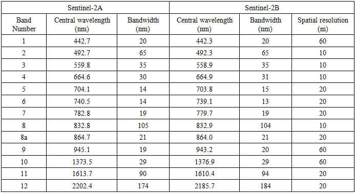
We employed satellite-sensed Sentinel 2, 10 m, spatial resolution, visible and NIR, ZCTA-stratified, LULC, capture point signature surveys of the potential epidemiological sampled county estimators. The combination of 10 m spectral bands [Table 1] enables a wide range of uses, including the monitoring of vegetation, soil, and water cover, and observing inland waterways and urban and rural areas in Hillsborough County. [9]Table 1. Sentinel-2 With 13 Spectral Bands at Different Spatial Resolutions: Four Bands at 10-Meter Resolution, Six Bands at 20-Meter Resolution, and Three Bands at 60-Meter Resolution
 |
| |
|
The digital overlay revealed the capture point, LULC-classified surface area (m2) of each epidemiological determinant in Hillsborough County. Land cover types were classified into urban commercial, urban residential, rural, farmland, and greenways.
2.4. Regression Model
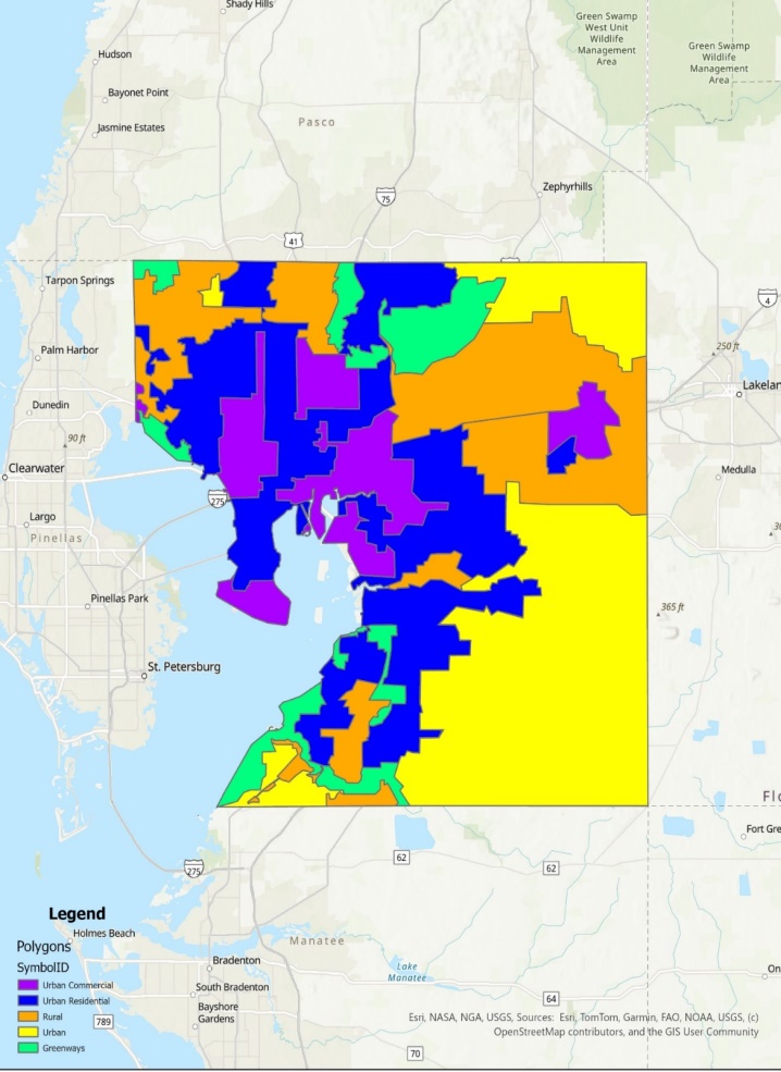 | Figure 1. Land Use Land Cover Map for Hillsborough County, Florida |
Initially, a Poisson regression with statistical significance was calculated at a 95% confidence level in R. The Poisson process in our analyses was provided by the limit of a binomial distribution of the epidemiological sampled county, ZCTA level, UC stratified estimator determinants, using 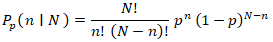 We viewed the distribution as a function of the expected number of the estimator determinant, UC, stratified, count variable, ZCTA, census, and online data in Hillsborough County using the sample size n for quantifying the fixed p in equation (2.1), which was subsequently transformed into the following equation:
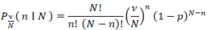 Based on the following sample size n, the distribution was solved using
 We generated plots and calculated the county ZCTA, Poisson distribution, which was also used to fit a generalized linear mixed model [GLMM] to the UC, stratified, data, capture points by maximum likelihood estimation (MLE) of the parameter vector β. While linear regression assumes a straight-line relationship and normally distributed outcomes, GLMMs can handle a variety of data types and distributions, making them suitable for real-world scenarios where data often deviates from these assumptions. [10] The procedure estimated the epidemiological sampled UC stratified parameters numerically through an iterative fitting process. The dispersion parameter was subsequently approximated by the quantified residual deviance and by Pearson’s chi-square divided by the degrees of freedom (d.f.). Pearson's chi-squared test is a statistical test applied to sets of categorical data to evaluate how likely it is that any observed difference between the sets arose by chance. which is the most widely used of many chi-squared tests (e.g., Yates, likelihood ratio, portmanteau test in time series, etc.). [11]For Pearson's chi-square testing of the UC estimator determinants, we employed
  to determine a chi-square distribution asymptotically. Covariances, standard errors, and p-values were computed using the stratified, estimator determinants based on the asymptotic normality derived from MLE in R. We used stratified UC estimators and relied on MLE with asymptotic normality, covariances, standard errors, and p-values, which were derived from the AN information matrix. We used the stratified Cox proportional hazards model:
  where:•
  socioeconomic, sociodemographic, and racial covariates •
  ZCTA-specific baseline hazard•
  common regression coefficients across ZCTA strataBaseline hazards differed by ZCTA, but regression effects
  was shared. Estimation was conducted by maximizing the stratified partial likelihood, which was computed as
  The log-likelihood:
  Under standard regularity conditions, we noted
  where
where  which was quantified using an observed Fisher information matrix. This result was the foundation for the covariances, standard errors, Wald tests, and p-values. The covariance matrix of
  was
was  . We derived the second derivatives of the stratified log-likelihood. We evaluated
  in the UC model. We inverted the information matrix. Likelihood was additive across ZCTA
  which we aere anble to determine using
  Standard error of the coefficient
  was subsequently quantified employing
  That was deciphered using the square root of the diagonal element of the inverse information matrix.We quantified the asymptotic normality in the UC model using:
  Under
Under  A two-sided p-value was determined by the models using:
 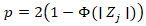 where
where  was the standard normal central density function [CDF]. The determinant of the information matrix:
  ten generated • Likelihood ratio tests• Asymptotic distribution derivations• Confidence region ellipsoids• Model comparison (AIC, etc.)For determining multivariate inference e we employed
 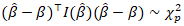 e: where
  was the number of parameters. We employed
  where:
  which was derived using
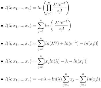 This was the sandwich estimator, robust t. Standard errors and p-values were then computed the same way but using this robust covariance matrix.We subsequently wrote the probability density function [PDF] of the Poisson distribution:
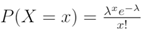 Next, we wrote the likelihood function. This was simply the product of the PDF for the observed, stratified, UC, ZCTA, racial, sociodemographic, and socioeconomic, epidemiological, sampled, estimator determinant, discrete integer values x1, …, xn. We subsequently calculated and generated the natural log likelihood function:We calculated the derivative of the natural log likelihood function with respect to λ in the UC model. Subsequently, we calculated the derivative of the natural log likelihood function with respect to the parameter λ in the model:
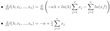 Thereafter, we set the derivative equal to zero and solved for λ in the model. Lastly, we set the derivative in the previous step equal to zero and simply solved for λ, which revealed
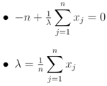 Hence, the MLE became:
 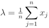 This was equivalent to the sample mean of the n sampled counties, ZCTA observations in the empirical UC stratified dataset. Next, wrote the likelihood function. This simply was a product of the PDF for the observed UC regressors values x1, …, xn.Note that the sample size n completely dropped out of the probability function, which in this experiment had the same functional form for all the capture points, sentinel site, stratified, racial, sociodemographic, and socioeconomic geosampled, estimator determinant, measurement, indicator, and discrete integer values. As expected, the Poisson distribution was normalized so that the sum of probabilities equaled 1. The ratio of probabilities was determinable by
 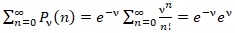 which was subsequently expressed as:
 Unfortunately, extra-Poisson variation was detected in the residual variance estimates in our model forecast. As such, we constructed a negative binomial regression model in R using a non-homogeneous gamma-distributed mean by incorporating
  in the equation. The prognosticative UC model distribution was then rewritten as
 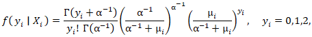 The negative binomial distribution was subsequently derived as a gamma mixture of Poisson random variables in the prognosticated UC regression county model. The conditional mean was
  and the conditional variance was
2.5. Spatial Autocorrelation
Next, a model was evaluated among the sampled stratified, racial sociodemographic, and socioeconomic covariates in Hillsborough County at the ZCTA level intervention sites using Moran’s I. In statistics, Moran's I is a measure of spatial eigen-autocorrelation. [12] We employed PySAL to compute Moran's I to detect stratified, CC hot and cold ZCTA-level, autocorrelated geolocations. We employed a weight matrix that represented the degree of relationship between the georeferenced ZCTA cells, for which we verified the latent zero and non-zero autocorrelation coefficients. We examined the residual autocovariance, which was arranged like a mosaic. We computed the weight matrix using the Contiguity-Based Weights method in PySAL. Contiguity-based weights are usable in eigen-spatial analysis to define neighboring observations by creating weight matrices, which express the connectivity between observations. [13] We started with a random matrix, Z. In our instance, the outcome of Moran's I approximated 0, serving as an effective test. Once we verified it worked efficiently with the random Z data, we substituted the model forecast with the epidemiological sampled UC data. An eigen-autocorrelation model specification was subsequently employed to describe the Poisson, random, county, ZCTA, stratified data. The resulting model specification took on the following form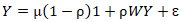 | (2.1) |
where μ was the scalar conditional mean of Y, and ε was an n-by-1 error vector whose elements were statistically independent and identically distributed (iid) normally random variates. The spatial covariance matrix for equation [2.1] employed the stratified, racial, sociodemographic and socioeconomic UC covariates in E [(Y - μ l)' (Y - μ l)] = Σ = [(I - ρ W')(I - ρ W)]-1σ2, where E (●) denoted the calculus of expectations, I was the n-by-n identity matrix delineating the matrix transpose operation, and σ2 was the error variance. Our assumption was that a mixture of latent, positive eigen-autocorrelation and negative eigen-autocorrelation may be present in the georeferenced, epidemiological, sampled, UC stratified, regression, model estimator determinants, which in turn we assumed would provide an even more explicit representation of the Poisson probability model results. Varying spatial, autoregressive parameters appeared in the covariance matrix, which, for our regression model specification, was describable employing | (2.2) |
The diagonal matrix of autoregressive parameters, <ρ >diag, contained two epidemiologically sampled UC parameters: ρ+ for those stratified, racial, sociodemographic, and socioeconomic covariates displaying positive eigen-spatial dependency, and ρ for those displaying negative eigen-spatial dependency. Since ρ+ = 0 (and hence I+ = 0 and I- = I) or ρ- = 0 (and hence I- = 0 and I+ = I), equation [2.2] reduces to equation [2.1]. This explanatory indicator variable classification was made in accordance with the quadrants of the corresponding Moran scatterplot generated using the scalable, ZCTA, CC, stratified, racial, sociodemographic, and socioeconomic, “Poisson’ covariates regressed in the county intervention ZCTA study sites.Neighbors based on contiguity were constructed by assuming that neighbors of a given georeferenced ZCTA area in Hillsborough County shared a common boundary. Neighbors can be of type Queen if a single shared boundary point meets the contiguity condition, or Rook if more than one shared point is required to meet the contiguity condition. [14] The function poly2nb() of the spdep package was employed to construct a list of georeferencable, stratifiable, ZCTA neighbors in Hillsborough County based on locations with contiguous boundaries, that is, georeferenced areas sharing one or more stratified capture points. We employed poly2nb() to calculate the neighbors of each of the regions of each intervention county based on Queen contiguity. The default type in poly2nb() is queen = TRUE, so neighbors of a given area are other areas. [15]Next, a spatially autoregressive (SAR) model specification was employed to describe the asymptotical, autoregressive variance in the estimates. An eigen-spatial filter model signature capture point specification was employed to describe both heterogeneous, Gaussian, and Poisson, random, stratifiable potential, hierarchical, diffusion-related, estimator determinant effects. The resulting SAR model specification took on the following form:  | (2.3) |
where μ was the scalar conditional mean of Y, and ε was an n-by-1 error vector whose elements were independently, identically distributed (i.d.d.) normalized random variates. The spatial covariance matrix for equation (2.3), fit the epidemiological sampled, eigen-decomposed UC, stratified i.d.d. covariates using E [(Y - μl)' (Y - μl)] = Σ = [(I - ρ W') (I - ρ W)]-1σ2, where E (●) denoted the calculus of expectations, I was the n-by-n identity matrix denoting the matrix transpose operation, and σ2 was the error variance. When a mixture of positive and negative latent eigen-autocorrelation is present in a non-time series, dependent, autoregressive vulnerability model, a more explicit representation of both effects leads to a more accurate interpretation of empirical results [20]. Alternatively, the excluded values were set to zero, and as such, the mean and variance had to be adjusted in the UC model. The model specification was subsequently transformed to | (2.4) |
where the diagonal matrix of the county ZCTA stratified UC parameters, < ρ >diag, contained the uncertainty-oriented, explanatory, autoregressive variables ρ+ for those determinants displaying positive eigen-spatial dependency, and ρ for those displaying negative eigen-spatial dependency. For instance, letting σ2 = 1 and employing a 2-by-2 regular square tessellation enabled positing a positive relationship between the eigen-autocorrelated covariates when y1 and y2, had a negative relationship between covariates, y3 and y4, and no relationship between covariates y1 and y3 and between y2 and y4. This covariance specification yielded:  | (2.5) |
when I+ was a binary 0-1, explanatory measurement indicator, county, ZCTA, stratified prognosticative inhomogeneous variable. The specification also denoted those epidemiological, sampled, uncertainty-free, normalized, exogenous predictors displaying positive eigen-spatial dependency when I- was a binary 0-1 variable, whilst denoting those estimator determinants displaying negative eigen-spatial dependency, employing I+ + I- = 1. If either ρ+ = 0 (and hence I+ = 0 and I- = I) or ρ- = 0 (and hence I- = 0 and I+ = I), then equation (2.5) reduces to equation (2.4). This indicator variable classification was made in accordance with the quadrants of the corresponding Moran scatterplot created using the stratified estimator determinants in PySAL.If positive and negative eigen autocorrelation processes counterbalance each other in a mixture, the sum of the two eigen-autocorrelation parameters--(ρ+ + ρ..) will be close to 0. [16] Here, Jacobian estimation was implementable by utilizing the non-homogeneous, diagnostic, explanatory, indicator values derived from the eigen-decomposed, eigen-spatial filtered exogenous variables (I+ - γ I-) in eigenvector eigen-geospace, which required estimating ρ+ and γ with ML techniques, and setting  An empirical eigen-autocorrelation weight matrix was generated for quantifying the autocovariance of the non-homoscedastic, multicollinear, zero autocorrelated, estimator determinants, which consisted of finding the normalized vectors ui stored as columns in the matrix U = [u1 ⋯ un]. This satisfied Λ = diag (λ1 ⋯ λ n),
  and
and  for i ≠ j. Note that double centering of Ω implied that the eigen-spatial filter, eigen-orthogonalized eigenvectors rendered from the exogenous regressors were centered, and at least one eigenvalue was equal to zero. Introducing these eigenvectors in the original formulation of Moran's I led to:
 | (2.6) |
The autocovariance is a function that gives the covariance of the process with itself at pairs of capture points, which is closely related to the eigen-autocorrelation [20]. We centered vector z = Hx and employed the properties of idempotence of H, which subsequently made the prognosticative, county, ZCTA, hot and cold spot, eigen-autocorrelation forecast model equivalent to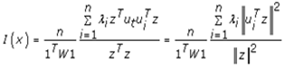 | (2.7) |
As the eigenvectors ui and the vector z were centered in the aggregation/non-aggregation-oriented, vulnerability-oriented, county, ZCTA hot and cold spot, regression model forecasts, equation (2.7) was rewritten: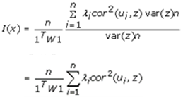 | (2.8) |
in PySAL, where n was the number of null eigenvalues of Ω (r ≥ 1). These eigenvalues and corresponding eigenvectors were removed from Λ and U, respectively. Equation (2.8) was strictly equivalent to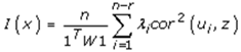 | (2.9) |
Moreover, it was demonstrated that Moran's I for a given UC-related eigen-spatial filter eigenvector ui was equal to I(ui) = (n/1T W1)λi, so the equation was rewritten 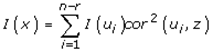 . The term cor2 (ui, z) represented the part of the variance of z that was explainable by ui in the county, ZCTA, hot/cold spot epidemiological model when z = β i ui+ ei. This quantity was equal to
  . By definition, the eigenvectors ui were eigen-orthogonal, and therefore, the UC regression coefficients of the linear models z = β i ui+ ei were those derivable from the regression model z = Uβ + ε = β iui + ⋯ + β n-r un-r + ε.The maximum value of 1 was quantifiable by all the variations of z, as parsimoniously expounded by the eigenvector u1, which corresponded to the highest eigenvalue λ1 in the weighted, autocorrelation, uncertainty-oriented matrix constructed from the estimator determinants. Here, cor2 (ui, z) = 1 (and cor2 (ui, z) = 0 for i ≠ 1) and the maximum value of I was intuitively deducible for Equation (2.9), which was equal to Imax = λ1(n/1TW1). The minimum value of I in the error matrix was obtainable as with all the variations of z, which in this experiment was definable by the eigenvector un-r corresponding to the lowest eigenvalue λn-r extractable in the model forecasts. This minimum value was equal to Imin = λn-r (n/1TW1). If the epidemiological sampled, explanatory, prognosticative, racial, interpolated socioeconomic, or sociodemographic variable was not definable due to the presence of heteroscedasticity, latent multicollinearity, and asymptoticalness in the epidemiological UC model forecasts, the part of the variance explained by each eigenvector was equal, on average, to cor2 (ui, z) = 1/n-1. Because the diagnostic, county, ZCTA, and capture point variables in z were randomly permuted, it was assumed that we would obtain this result.The observed and expected numbers of the racial sociodemographic and socioeconomic determinants were denoted by Y = (Y1, …, Yn) and E = (E1, …, En), respectively. In addition, we denoted the matrix of p [i.e., intervention, stratified UC covariate] as a column of ones for the intercept term, where the epidemiologically sampled discrete integer values related to a ZCTA in Hillsborough County, β = (β0, β1, …, βp) denoted the vector of the covariate effects, whilst Rk represented the UC risk at a georeferenced ZCTA location. A value of Rk greater (less) than one indicated that the ZCTA had a higher (lower) than average UC risk, and in terms of interpretation.
3. Results
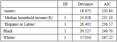
Stepwise Backward was used. Whites, Blacks, Hispanics, and median household income were most relevant.Table 2. Stepwise Backward Results
 |
| |
|
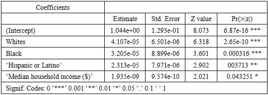
Table 3. Poisson Results Summary
 |
| |
|
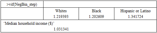
Table 4. Variance Inflation Factor Values
 |
| |
|
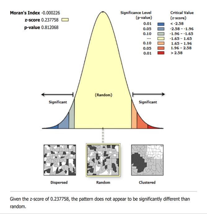 | Figure 2. Spatial autocorrelation report for modeled uterine cancer vulnerability across Hillsborough County ZCTA regions using Moran’s I statistics and eigen-spatial filtering procedures |
 | Figure 3. Global Moran’s I summary for modeled uterine cancer vulnerability across Hillsborough County ZCTA regions. Spatial autocorrelation significance was evaluated using permutation-based inference (999 permutations; α = 0.05). Positive Moran’s I values indicate clustering of similar vulnerability estimates |
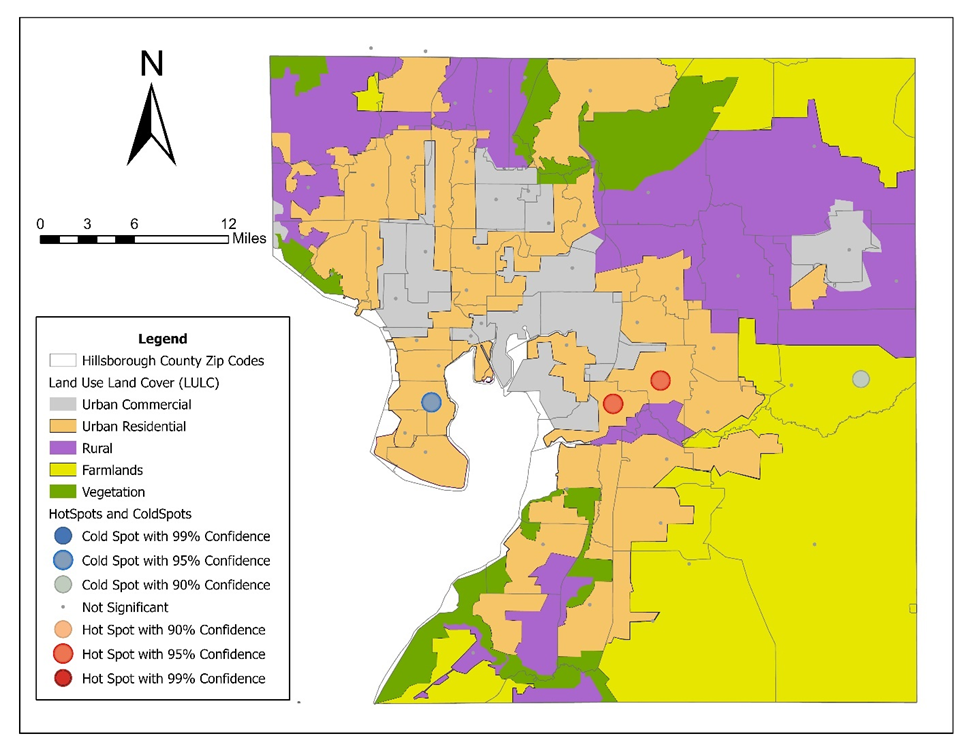 | Figure 4. Hot and cold spot maps for modeled uterine cancer vulnerability in Hillsborough County, Florida. Statistically significant clustering patterns were identified using Moran’s I spatial autocorrelation procedures and eigen-spatial filtering methods. Hot spots represent higher-than-expected modeled vulnerability regions, whereas cold spots represent lower-than-expected modeled vulnerability regions |
4. Discussion
Our mathematical modeling of uterine health outcomes at moderate spatial resolution—specifically the identification of “hot” and “cold” spots at the ZCTA level—required the integration of spatial statistics, stochastic processes, and covariate-informed regression within a unified framework for capturing both structured heterogeneity and latent risk. To achieve this, we incorporated spatially correlated random effects to account for geographic dependence while allowing for unobserved variation across neighboring regions. The model also leveraged techniques to borrow strength across ZCTA, improving stability in areas with sparse data. Together, this approach provides a robust, data-driven basis for identifying high-risk areas and informing targeted public health interventions for uterine cancer prognosticative vulnerability modelling at the ZCTA level.Initially, we let  index ZCTA regions, and let
  denote an observed uterine-related outcome, [ number of cases] associated with uterine cancer. The observed counts
  were assumed to follow a Poisson or negative binomial distribution,
  , with intensity
  , where
  represented an offset (e.g., expected cases given population) and
  was the relative risk. The log-risk was expressible as a structured additive predictor,
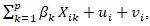 where
where  encoded sociodemographic, socioeconomic, and racial covariates—such as educational attainment, racial composition etc.—and
  represented spatially structured and unstructured random effects, respectively. The structured component was then modeled via a conditional autoregressive (CAR) prior,
 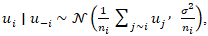 where adjacency
  reflects ZCTA contiguity, thereby enforcing spatial smoothness and enabling the emergence of localized uterine outcome–stratified clusters. This specification was further extended to the intrinsic CAR (ICAR) formulation by expressing the joint distribution as a Gaussian Markov random field with precision structure,
  where
where  was the binary adjacency matrix and
  was the diagonal matrix of neighbor counts, ensuring that borrowing of strength occurs proportionally to spatial connectivity. To accommodate overdispersion and unmeasured confounding, the structured CAR term was combined with an unstructured heterogeneity component, yielding a Besag–York–Mollié (BYM) specification:
  where
where  denoted the latent risk on the log-scale and
  represented covariates capturing socioeconomic, racial, and sociodemographic predictors. Posterior inference was conducted within a hierarchical Bayesian framework, enabling simultaneous estimation of fixed effects and spatial random effects while quantifying uncertainty in cluster identification. This formulation allows the model to distinguish persistent high-risk “hot spots” from transient spatial noise by exploiting the joint dependence structure encoded in the precision matrix
  . The resulting posterior risk surfaces were interpretable as smoothed estimates of underlying uterine cancer intensity, facilitating principled hot and cold spot detection through exceedance probabilities, e.g.,
  . The CAR models were represented via eigenfunction/eigen-decomposition of the graph Laplacian, which gave strong intuition (CAR = smoothing over low-frequency eigenmodes). But in computation, the uterine cancer prognosticative CAR models are implemented via sparse precision matrices rather than explicit spectral decomposition.Hot and cold spot models of vulnerability can formally identify uterine cancer at the ZCTA level through posterior exceedance probabilities
  and
and  , respectively, with thresholds (e.g., 0.95) for delineating statistically significant high- and low-risk regions. An alternative but complementary formulation for ZCTA uterine cancer modelling arises from spatial scan statistics, in which one defines a likelihood ratio test over moving spatial windows
  maximizing
  where
where  and
and  denote observed and expected counts within the candidate cluster; this approach, developed in Kulldorff’s spatial scan framework, provides a frequentist mechanism for detecting spatial concentration without explicit prior assumptions, which may apply to uterine cancer vulnerability modelling. [17] To incorporate temporal evolution and potential non-stationarity, a uterine cancer researcher or epidemiologist may extend the model to a spatio-temporal stochastic differential system
  or, more practically, a discrete-time dynamic formulation
  , where
  , thereby allowing evolving disparities tied to shifting socioeconomic conditions. To further capture the latent dynamics in a ZCTA prognosticative uterine forecast model, it can be augmented with an autoregressive structure such a
  which enables the gradual propagation of risk over time rather than abrupt temporal shifts. This formulation may permit the separation of long-term structural heterogeneity from short-term shocks through the decomposition of
  where
where  may encode stable spatial effects and
  capture transient deviations. In addition, interaction terms of the form
  may be included to explicitly model time-varying covariate effects, allowing socioeconomic, racial, and sociodemographic gradients to exert increasing or diminishing influence over the study horizon. Within a hierarchical framework, such extensions may naturally integrate with CAR-based spatial priors to yield a full spatio-temporal Gaussian Markov random field, enabling coherent inference on both evolving risk surfaces and their associated uncertainty for optimizing uterine cancer forecast vulnerability modelling.A fundamentally different yet increasingly prominent alternative is the use of machine learning architectures for spatial prediction, wherein the risk surface is approximated by a nonlinear function
  with
with  encoding spatial coordinates or graph embeddings derived from ZCTA adjacency; graph neural networks, for instance, implement updates of the form
  thereby learning spatial dependencies directly from the data [20]. These models may allow interpretability necessary for public health policy, particularly when disentangling the effects of race, sociodemographic, and socioeconomic status, which may be confounded through structural inequities. Agent-based models provide yet another complementary perspective, simulating individuals with attributes
  interacting within ZCTA-defined environments, where transition probabilities for uterine cancer progression may depend explicitly on access to care, environmental exposures, and behavioral factors; however, these models require detailed microdata to calibrate at scale.Across these frameworks, the inclusion of racial, sociodemographic, and socioeconomic covariates must be handled with conceptual and statistical care, as coefficients
  may reflect not intrinsic biological differences but rather systemic disparities in healthcare access, environmental exposure, and structural inequality. [18], [19] Consequently, uterine model interpretation should emphasize conditional associations rather than causal attribution unless supported by appropriate identification strategies. In synthesis, hierarchical spatial models with CAR priors, augmented by temporally adaptive structures such as GARCH processes, may provide a particularly powerful and flexible approach for identifying ZCTA–level hot and cold spots in uterine health outcomes, balancing interpretability, statistical rigor, and the capacity to incorporate rich covariate information, while alternative approaches—scan statistics, stochastic dynamics, and machine learning. This would offer complementary strengths in detection, temporal modeling, and predictive performance. Several limitations should be acknowledged. First, directly observed uterine cancer prevalence data were unavailable at the ZCTA level; therefore, modeled small-area estimates were constructed using county-level incidence data combined with demographic stratification procedures. As such, the resulting hot spot and cold spot surfaces represent exploratory spatial vulnerability approximations rather than definitive disease prevalence measurements. Second, ecological interpretation at the ZCTA level may not fully capture individual-level heterogeneity or causal mechanisms underlying uterine cancer disparities. Despite these limitations, the framework remains useful for exploratory spatial epidemiology and geographically targeted public health planning under incomplete surveillance conditions.
5. Conclusions
The identification of uterine cancer stratified hot and cold spots at the ZCTA level through mathematically rigorous frameworks underscores the necessity of integrating spatial dependence, stochastic variability, and covariate-informed structure within a coherent modeling paradigm. Hierarchical spatial models, particularly those incorporating conditional autoregressive priors, can provide a principled balance between interpretability and flexibility, enabling the estimation of localized relative risks while accounting for both spatial autocorrelation and heteroskedasticity. Spatial statistics, spatio-temporal stochastic models, and graph-based machine learning architectures offer complementary advantages in uterine cancer cluster detection, dynamic forecasting, and high-dimensional pattern recognition. Crucially, the inclusion of socioeconomic, sociodemographic, and racial covariates can be interpreted within the broader context of structural inequities, as observed disparities in conditions such as uterine fibroids and endometrial cancer reflecting differential access to care, environmental exposures, and systemic bias rather than purely biological variation. Accordingly, the ultimate value of these models lies not only in their statistical precision but in their capacity to inform equitable, geographically targeted interventions, reinforcing the role of advanced spatio-temporal mathematical modeling in precision public health.
ACKNOWLEDGEMENTS
N/A
DISCLOSURE
N/A
References
| [1] | J. D. Wright, M. T. Prest, J. S. Ferris, et al. Projected trends in the incidence and mortality of uterine cancer in the United States. Cancer Epidemiol Biomarkers Prev. 2025; 34(7): 1156-1166. |
| [2] | D. A. Griffith. Spatial Autocorrelation and Spatial Filtering: Gaining Understanding Through Theory and Scientific Visualization. New York, NY: Springer; 2003. |
| [3] | A. Satardekar, J. Liu, H. McDonald, B. Jacob. Employing Markov chain Monte Carlo (MCMC) Bayesian Poissonian and a second-order eigenfunction eigendecomposition algorithm to geostatistically target landscape covariates associated with leukemia in Hillsborough County, Florida. Br J Healthc Med Res. 2024; 11(4). |
| [4] | K. Eaton, A. Satardekar, N. Choudhari, R. Shah, B. G. Jacob. Decomposition of Moran’s coefficient to detect nonmulticollinear, non-zero, eigen-autocorrelated, non-Gaussian coefficients in colorectal cancer estimator determinants epidemiologically sampled in Hillsborough County, Florida. Ann Biostat Biometric Appl. 2026; 7(2): 1-11. |
| [5] | U.S. Census Bureau. QuickFacts: Hillsborough County, Florida. Accessed April 23, 2026. https://www.census.gov/quickfacts/fact/table/hillsboroughcountyflorida/PST045224. |
| [6] | U.S. Census Bureau. Hillsborough County, Florida: Population Characteristics (Population, Age, Sex, Race, and Housing Data). Accessed April 23, 2026. https://data.census.gov/profile/Hillsborough_County,_Florida?g=050XX00US12057#populations-and-people. |
| [7] | U.S. Census Bureau. Hillsborough County, Florida: Census Data Profile. Accessed April 23, 2026. https://data.census.gov/profile/Hillsborough_County,_Florida?g=050XX00US12057. |
| [8] | National Cancer Institute. State Cancer Profiles: Incidence Rates by County (Florida). Accessed April 23, 2026. https://statecancerprofiles.cancer.gov/incidencerates/index.php?statefips=12&areatype=county&cancer=058& race=00&age=001&stage=999&ruralurban=0&type=incd&sortVariableName=rate&sortOrder=default&output =0. |
| [9] | K. K. Ritchie, R. Izurieta, I. Hoare, et al. Mapping Aedes aegypti bird bath habitats for implementing “seek and destroy” larval source management in Hillsborough County, Florida, USA. American Journal of Entomology. 2024; 8(1): 1-17. |
| [10] | D. W. Hosmer, S. Lemeshow, Applied Logistic Regression. 2nd ed. John Wiley & Sons; 2000. |
| [11] | P. E. Greenwood, M. S. Nikulin. A Guide to Chi-Squared Testing. New York, NY: Wiley; 1996. |
| [12] | D. A. Griffith. Spatial Autocorrelation and Spatial Filtering: Gaining Understanding Through Theory and Scientific Visualization. New York, NY: Springer; 2003. |
| [13] | D. A. Griffith. Spatial Autocorrelation and Spatial Filtering. Berlin, Germany: Springer; 2003. |
| [14] | D. A. Griffith. Spatial Autocorrelation and Spatial Filtering. Berlin, Germany: Springer; 2003. |
| [15] | D. A. Griffith. Spatial Autocorrelation and Spatial Filtering. Berlin, Germany: Springer; 2003. |
| [16] | D. A. Griffith. Spatial Autocorrelation and Spatial Filtering: Gaining Understanding Through Theory and Scientific Visualization. New York, NY: Springer; 2003. |
| [17] | M. Kulldorff. A spatial scan statistic. Commun Stat Theory Methods. 1997; 26(6): 1481-1496. |
| [18] | A. V. Diez Roux. A glossary for multilevel analysis. J Epidemiol Community Health. 2002; 56(8): 588-594. |
| [19] | N. Krieger. Methods for the scientific study of discrimination and health: An ecosocial approach. Am J Public Health. 2012; 102(5): 936-944. |
| [20] | Jacob, B. G., Izurieta, R., Bell, J., Parikh, J., Loum, D., Casonova, J., Gates, T., Murray, K., White, L., & Aceng, J. R. (2023). Approximating non-asymptoticalness, skew heteroscedasticity, and geo-spatiotemporal multicollinearity in posterior probabilities in Bayesian eigenvector eigen-geospace for optimizing hierarchical diffusion-oriented COVID-19 random effect specifications geosampled in Uganda. American Journal of Mathematics and Statistics, 13(1), 1–43. https://doi.org/10.5923/j.ajms.20231301.01. |

 Abstract
 Reference
 Full-Text PDF
 Full-text HTML