Shradha Patil, Sharada V. Bhat
Department of Statistics, Karnatak University, Dharwad, India
Correspondence to: Sharada V. Bhat, Department of Statistics, Karnatak University, Dharwad, India.
| Email: |  |
Copyright © 2024 The Author(s). Published by Scientific & Academic Publishing.
This work is licensed under the Creative Commons Attribution International License (CC BY).
http://creativecommons.org/licenses/by/4.0/

Abstract
Control charts are widely used in quality control to monitor and detect changes in the process location and variability. In this paper, we present a control chart based on Gastwirth estimator for monitoring the process location. The performance of the proposed control chart is evaluated through various performance measures providing a comprehensive analysis of its shift detection capability. The proposed control chart is compared with its competitors. The control chart is demonstrated through an example to showcase its application in reality.
Keywords:
Control limits, Gastwirth estimator, Median run length, Order statistic, Outliers, Process location
Cite this paper: Shradha Patil, Sharada V. Bhat, Process Location Control Chart based on Gastwirth Estimator, American Journal of Mathematics and Statistics, Vol. 14 No. 2, 2024, pp. 33-41. doi: 10.5923/j.ajms.20241402.02.
1. Introduction
Control charts are vital tools in statistical quality control, offering a visual means of monitoring process parameters over time. They enable practitioners to distinguish between chance and assignable causes of variation, which signals potential issues that require intervention. By continuously monitoring process mean and variance, control charts facilitate timely decision-making and help maintain quality products. Specifically, control charts for monitoring process location are crucial for ensuring that the mean of a process remains stable over time. The early work of Shewhart (1931) laid the foundation for control charts which assume normality and utilize 3-sigma control limits to detect shifts in process mean. Page (1961) introduced cumulative sum control charts (CUSUM) which are sensitive to detect small shifts in the process mean. Roberts (1959) proposed exponentially weighted moving average (EWMA) control chart which assigns weights to previous observations, making it more sensitive to detect small shifts. Montgomery (1996) provides a comprehensive overview of control charts, discussing various types of control charts, their underlying concepts and applications in monitoring process stability in detecting shifts in process parameters.Many control charts for process location parameter rely on the assumption that the underlying process has normal distribution. However, in practice, this assumption need not be valid. For example, in glass industry, the thickness of glass sheets used for windows, screens or optical applications is critical to monitor the process parameter. The thickness measurements are often symmetrically distributed around a target value due to production techniques like the float glass process. Some slight variations in the cooling process or other external factors can result in occasional extreme deviations which lead to a heavy-tailed distribution, where control charts based on normality may fail to detect these changes.As a result, it is essential to propose control charts that do not rely on the assumption of normal distribution. To address this issue, it is necessary to develop control charts that are resilient to non normality. Some significant studies that do not rely on the assumption of normality include control charts based on sign statistics proposed by Amin et al. (1995), distribution-free Shewhart type control chart based on signed ranks developed by Bakir (2004), synthetic control chart developed by Pawar and Shirke (2010), Shewhart type nonparametric control chart based on the run statistic suggested by Zombade and Ghute (2019). A comprehensive overview of nonparametric control charts, detailing various methodologies for quality control is studied by Chakraborti (2019). Here, the author emphasizes the robustness and applicability of nonparametric approaches in statistical process control providing practical insights and examples for practitioners. Bhat and Patil (2024a and 2024b) propose control charts for process location based on sample median and sample midrange respectively to monitor the process location parameter, employing Shewhart's methodology. In this paper, we propose a control chart that employs a robust statistical measure to improve monitoring accuracy and enhance shift detection in process location, especially in the presence of outliers and under non normal distributions. Section 2 deals with proposed control chart and section 3 discusses the evaluation of proposed control chart. In sections 4 and 5, we respectively deal with illustration of the proposed control chart through examples and conclusions based on our observations.
2. Control Chart Based on Gastwirth Estimator
In this section, we propose control chart based on Gastwirth estimator (G) due to Gastwirth (1966) which is a robust estimator. Suppose  is a random sample of size
  from a distribution with cumulative density function
  , then G is given by
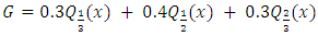 | (1) |
where  is
is  sample quantile.Also, suppose
  represents
  order statistic, then
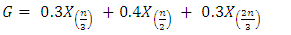 | (2) |
where  and
and  represent 33rd, 50th and 66th percentiles of the data. The estimator is useful from practical point of view as it has better efficiency than median and is also robust. It has better computational efficiency than other robust estimators like estimators due to Harrel and Davis (1982) and Hodges and Lehmann (1963). Also, it is helpful in estimating the location parameter in the presence of outliers or when process has non-normal distribution. Its approach of using fixed weights enable its utility across various symmetric distributions.According to DasGupta (2008), G has asymptotically normal distribution with mean
 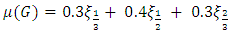 | (3) |
and variance  , where
  and
and  are respectively the population quantiles corresponding to the 33rd, 50th and 66th percentiles.
 | (4) |
where 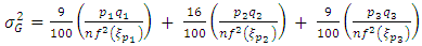
 ,for
,for  with
with  and
and  for
for  . Here,
  and
and  is value of density function at the specified population quantile
  Therefore,
 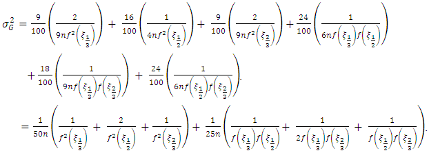 | (5) |
The variance expression captures the estimator's variability as a function of the sample size  and the values of the density function
  at the specified population quantiles
  and
and  Under the assumption that, a random sample of size
  is taken from a symmetric or skewed distribution with location parameter
  and scale parameter
  , following Shewhart (1931), we propose G control chart
  | (6) |
 | (7) |
 | (8) |
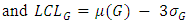
where  and
and  are respectively upper control limit, centre line and lower control limit of G control chart. And
  is standard deviation
  of G.
of G.
3. Performance of G Control Chart
In this section, we evaluate the performance of the G control chart for various distributions under consideration. To assess the performance of the proposed G control chart, we compute mean and  of G control chart under uniform (U), exponential (E), normal (N), logistic (LG), Laplace (L) and Cauchy (C) distributions. The distributions are modified in terms of
  and
and  such that they have mean
  and variance
  . As G approximately follows normal distribution with mean
  and
and  given by square root of (5), we have to evaluate
  and
and  under various distributions. For example, to evaluate
  under exponential distribution,
 | (9) |
 | (10) |
 | (11) |
Substituting (11) in (9), we get  | (12) |
On similar lines, other values of  in (5) are evaluated and
  is obtained. The
  and width
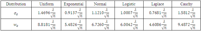
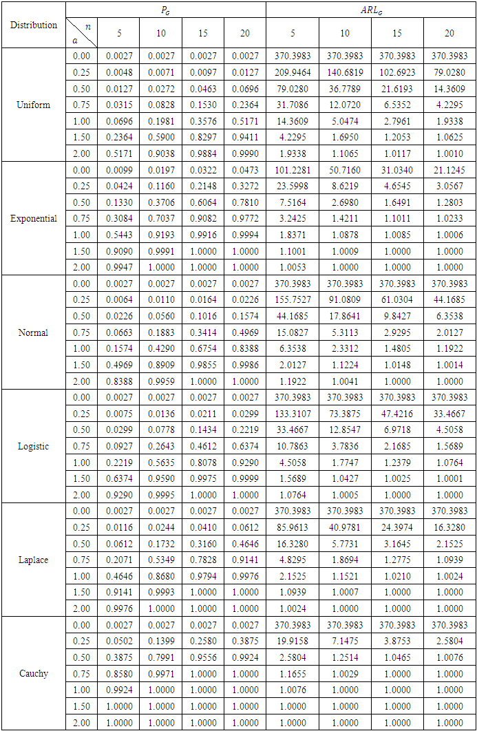
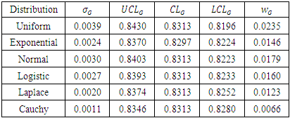
  of G control chart for the distributions under consideration is furnished in Table 1.
Table 1.
 of G control chart for various distribtions of G control chart for various distribtions
 |
| |
|
The  of the G estimator varies across distributions based on their differences in spread and tail behavior. The G statistic under Cauchy distribution has highest
  and under Laplace distribution has lowest
  . The width of G control chart is highest for Cauchy distribution followed by uniform distribution and is lowest for Laplace distribution followed by exponential distribution. To evaluate the performance of G control chart, we consider various performance measures such as power
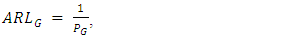
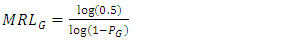
  , average run length
  median run length
  and standard deviation of run length
  . These measures provide a comprehensive view of the control chart’s ability to detect shifts in the process location. The
  refers to the probability,
  represents the expected number of samples required and
  gives the median number of samples needed to detect a shift in process location. A smaller
  and
and  value indicates quicker detection of shifts. Additionally, the
  evaluates the consistency of shift detection, where a lower value indicates better consistency. Various measures are given by
 | (13) |
 | (14) |
 | (15) |
 | (16) |
 | (17) |
The values of  and
and  for uniform, exponential, normal, logistic and Laplace distributions are determined by setting
  and for Cauchy distribution by setting
  due to Arnold (1965). For sample sizes
  and various positive shifts, the computed values of
  are provided in Table 2 and
 are provided in Table 3.
  and
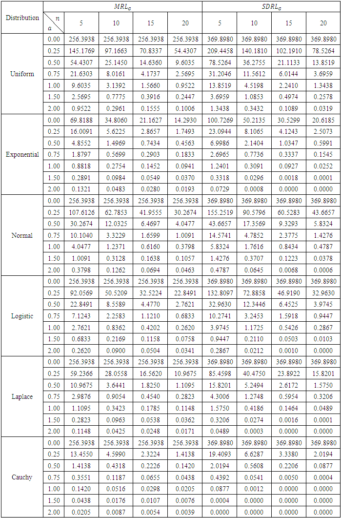
and  of G control chart are plotted in Figure 1 for
  .
.Table 2.
 for various distributions for various distributions
 |
| |
|
Table 3.
 for various distributions for various distributions
 |
| |
|
 | Figure 1.  of G Control Chart of G Control Chart |
From Table 2 and 3, for all values of  we observe that,
  is 0.0027 for symmetric distributions under consideration at zero shift. However, since
  for exponential distribution,
  is
is  at
at  . The
. The  increases as
  and
and  increase. For fixed
  and small
  is highest for Cauchy distribution and lowest for uniform distribution. We notice that, under symmetric distributions,
  and
and  are approximately 370 and 256 respectively for zero shift. Under exponential distribution, these values are achieved at
  . Also,
  and
and  being smaller, vary for different
  for zero shift. For fixed
  , as
, as  increases,
  and
and  decrease, exhibiting effective shift detecting capability of the control chart. The same nature in
  and
and  is observed for fixed
  and increasing
  . Also,
  decreases for increasing
  and
and  , indicating stability of the control chart in detecting the shifts.From Figure 1, it is observed that, among symmetric distributions, for specified value of
  , both
  and
and  decrease across uniform distribution to Cauchy distribution. Hence, if the process variables are from uniform distribution, G control chart is less sensitive in detecting smaller shifts, whereas, it reflects strong sensitivity to detect shifts under heavier tailed distributions like Laplace and Cauchy distributions. Under exponential distribution, though
  and
and  are decreasing for smaller shifts, the detection of shift could be illusive since these values are smaller at zero shift itself. On comparing the G control chart with median (M) control chart due to Bhat and Patil (2024a), in terms of ARL, we observe that,
  is lower than
  under uniform, normal and logistic distributions, whereas,
  is higher than
  for Laplace distribution. These values are almost same under Cauchy distribution. This indicates that, G control chart detects shifts in the process location quickly than the M control chart when process has uniform, normal, logistic distributions and has almost equal efficiency when process has Cauchy distribution. As G curtails 29% outliers and M curtails 50% outliers, G control chart is less resilient than M control chart to outliers. Here, G control chart is better than M control chart when process variables are from light and medium tailed distributions. However, it is equally competitive when process variables have heavy tailed distributions.
4. Illustration
In this section, we illustrate G control chart with two examples given in Duncan (1955) and Ghute and Shirke (2008).Example 1: The example due to Duncan (1955) deals with the height (inches) of fragmentation of bomb base that consists of 5 samples taken 29 times and is given in Table 4. The  , control limits and width of G control chart is given in Table 5. Figure 2 is plotted using Table 4 and Table 5.
Table 4. Height (inches) of fragmentation of bomb base and computed values of G,

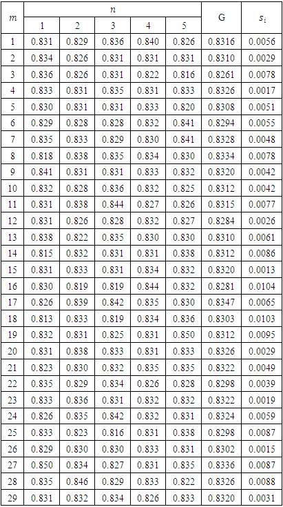 |
| |
|
Table 5.
 under various distributions under various distributions
 |
| |
|
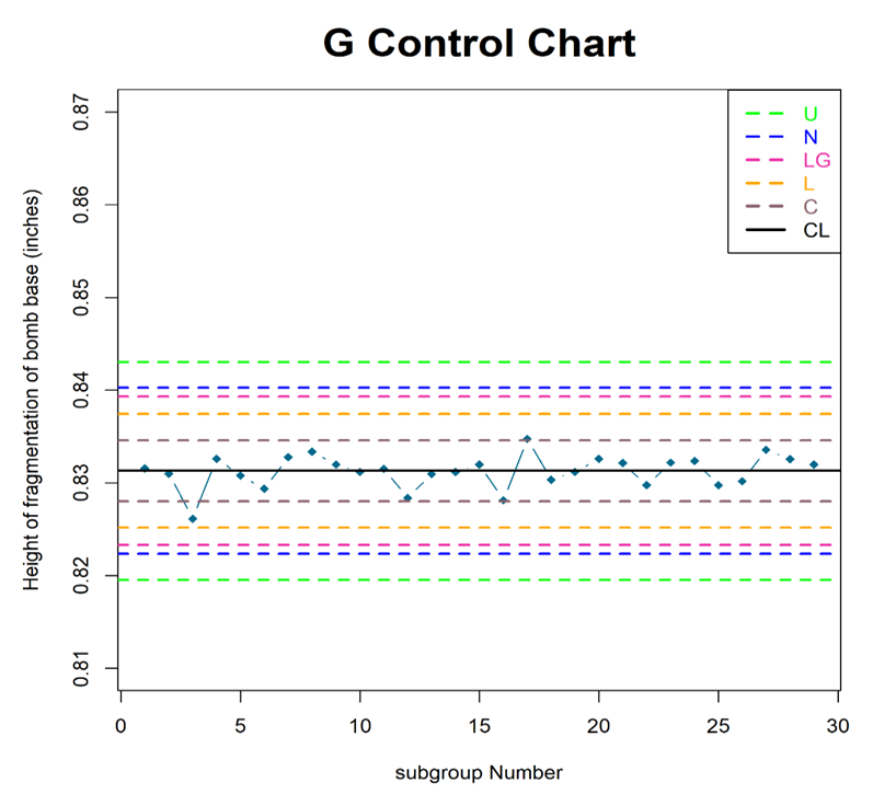 | Figure 2. G control chart for symmetric distributions |
Since  and
and  are unknown, they are estimated from the samples. Suppose
  samples are taken
  times,
  is estimated by taking the weighted average of 33rd, 50th and 66th percentiles of the samples, with weights respectively given by 0.3, 0.4 and 0.3. That is,
  where
where 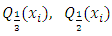 and
and  is 33rd, 50th and 66th percentiles of the of
  sample. And
  is estimated by obtaining
  under various distributions by substituting
  where
where 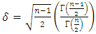 for λ. Here
  where
where  . For
. For  .From Table 5 and Figure 2, we observe that,
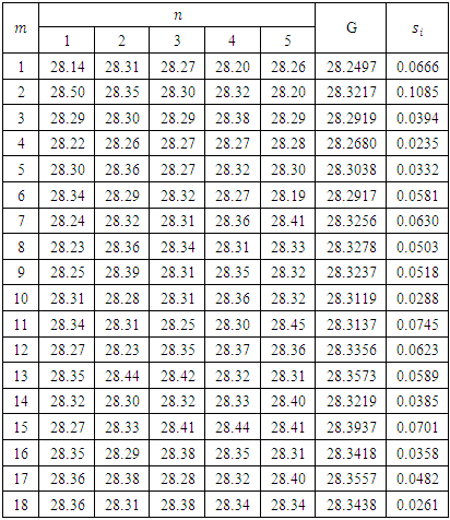
  is narrower for Cauchy distribution, whereas, it is wider for uniform distribution. The centre line of exponential distribution differs from that of symmetric distribution. From Figure 2, we see that, the process is out of control for Cauchy distribution, whereas, it exhibits in control status under other symmetric distributions.Example 2: The partial data is taken from Ghute and Shirke (2008) which is due to Chen et al. (2005). The data consists of 5 samples taken 18 times from a spring manufacture process. The measurements of the inner diameter of the springs are given in Table 6 and
  , control limits,
  are given in Table 7. Figure 3 is plotted using Table 6 and Table 7. The computations are carried out on similar lines of example 1.
Table 6. Springs inner diameter and computed values of G,

 |
| |
|
Table 7.
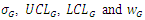 under various distributions under various distributions
 |
| |
|
 | Figure 3. G control chart for symmetric distributions |
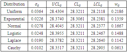
From Table 7 and Figure 3, we observe that,  becomes narrower for heavier tailed distributions. The centre line of all symmetric distributions is the same, whereas, it is different for exponential distribution. From Figure 3, we notice that, process is out of control under Cauchy and Laplace distributions, while it remains in control under other symmetric distributions.
5. Conclusions
In this section, based on our findings, we record our conclusions on the proposed G control chart. • A control chart based on Gastwirth estimator (G) has been proposed for monitoring process location under the assumption that, the process variables have cumulative density function,  .• The
  of G estimator is obtained and the control limits of the proposed control chart is developed under various symmetric and asymmetric distributions.• The proposed control chart is evaluated using various performance measures viz. power, ARL, MRL and SDRL for different shifts and sample sizes.• Power of the G control chart is high for Cauchy distribution as compared to other distributions.• ARL and MRL decrease for smaller shifts and sample sizes under heavy tailed distributions like Laplace and Cauchy distributions.• The proposed control chart has lucidity in detecting the shifts in the process location under Cauchy model.• The G control chart outperforms M control chart due to Bhat and Patil (2024a), when process variables have uniform, normal, logistic distributions and equally performs under Cauchy distribution.• The proposed control is deplorable under skewed distribution like exponential distribution as the detection of shifts by control chart could be misleading.• The G control chart is useful when the distributional assumption of normality is not valid. Also, it is highly desirable when process variables are from heavy tailed distributions.
ACKNOWLEDGEMENTS
Authors thank the unknown referee whose suggestions have been useful in improvisation of the paper.
References
| [1] | Amin, R. W., Reynolds, M. R. and Saad, B. 1995. Nonparametric quality control charts based on the sign statistic. Communications in Statistics - Theory and Methods, 24(6), 1597–1623. https://doi.org/10.1080/03610929508831574. |
| [2] | Arnold, H. J. 1965. Small sample power of the one sample Wilcoxon test for non-normal shift alternatives. The Annals of Mathematical Statistics, 1767-1778. http://dx.doi.org/10.1214/aoms/1177699805. |
| [3] | Bakir, S. T. 2004. A distribution-free Shewhart quality control chart based on signed-ranks. Quality Engineering, 16(4), 613-623. https://doi.org/10.1081/QEN-120038022. |
| [4] | Bhat, S. V. and Patil, S. 2024b. Midrange control chart under non normality. Global Journal of Pure and Applied Mathematics. 20. 169-182. DOI:10.37622/GJPAM/20.1.2024.169-182. |
| [5] | Bhat, S. V. and Patil, S. S. 2024a. Shewhart type control chart based on median for location parameter. International Journal of Agricultural & Statistical Sciences, 20(1). |
| [6] | Chakraborti, S. and Graham, M. 2019. Nonparametric statistical process control. John Wiley & Sons. |
| [7] | Chen, G., Cheng, S. W. and Xie, H. 2005. A new multivariate control chart for monitoring both location and dispersion. Communications in Statistics—Simulation and Computation®, 34(1), 203-217. DOI: 10.1081/SAC-200047087. |
| [8] | DasGupta, A. 2008. Asymptotic theory of statistics and probability (Vol. 180). New York: Springer. |
| [9] | Duncan, A. J. 1955. Quality control and industrial statistics. RD Irwin. |
| [10] | Gastwirth, J. L. 1966. On robust procedures. Journal of the American Statistical Association, 61(316), 929-948. https://doi.org/10.1080/01621459.1966.10482185. |
| [11] | Ghute, V. B. and Shirke, D. T. 2008. A multivariate synthetic control chart for monitoring process mean vector. Communications in Statistics—Theory and Methods, 37(13), 2136-2148. DOI: 10.1080/03610920701824265. |
| [12] | Harrell, F. E. and Davis, C. E. 1982. A new distribution-free quantile estimator. Biometrika, 69(3), 635-640. https://doi.org/10.1093/biomet/69.3.635. |
| [13] | Hodges, J.L. and Lehmann, E.L. 1963. Estimates of Location Based on Rank Tests. Annals of Mathematical Statistics, 34, 598-611. https://www.jstor.org/stable/2238406. |
| [14] | Montgomery, D. C. 1996. Introduction to statistical quality control (6th Edition ed.). John Wiley & Sons. |
| [15] | Page, E. S. 1961. Cumulative sum charts. Technometrics, 3(1), 1-9. https://doi.org/10.2307/1266472. |
| [16] | Pawar, V. Y. and Shirke, D. T. 2010. A nonparametric Shewhart-type synthetic control chart. Communications in statistics-Simulation and Computation, 39(8), 1493-1505. https://doi.org/10.1080/03610918.2010.503014. |
| [17] | Roberts, S.W. 1959 Control Chart Tests Based on Geometric Moving Averages. Technometrics, 1, 239-250. http://dx.doi.org/10.1080/00401706.1959.10489860. |
| [18] | Shewhart, W. A. 1931. Statistical method from an engineering viewpoint. Journal of the American Statistical Association, 26(175), 262-269. |
| [19] | Zombade, D. M. and Ghute, V. B. 2019. Shewhart-type nonparametric control chart for process location. Communications in Statistics-Theory and Methods, 48(7), 1621-1634. https://doi.org/10.1080/03610926.2018.1435811. |

 Abstract
 Reference
 Full-Text PDF
 Full-text HTML