1. Introduction

Volatility modeling of stock market returns has been gaining great interest by financial markets participants, academia, financial analysts and the general public. Volatility measures the uncertainty and risk which play significant role in modern financial analysis. Measuring and predicting volatility is crucial for financial decision making and has significant applications in areas such as portfolio selection, option pricing, risk management, hedging and strategic pair-trading as well as Value-at-Risk (VaR) estimation. Providing accurate volatility estimates in Nigeria market avails regulators, government, traders and investors the opportunity to formulate better policies and make appropriate financial investment decisions, (Emenike, 2010). Modelling volatility is an important element in pricing equity, risk management and portfolio management. Stock prices reflect all available information and the quicker they are in absorbing accurately new information, the more efficient is the stock market in allocating resources. Modelling volatility will improve the usefulness of stock prices as a signal about the intrinsic value of securities, thereby, making it easier for firms to raise fund in the market. Also, detection of stock returns volatility-trends would provide insight for designing investment strategies and for portfolio management. The accuracy of volatility estimates and the precision of interval forecast is compromised if structural breaks are ignored (Orabi and Alqurran, 2015; Adewale et al., 2016; Kuhe and Chiawa, 2017). Studies conducted by Perron (1989, 1990)); Diebold and Inoue (2001); Gil-Alana et al. (2015), among others, revealed that when stationary processes are contaminated with structural breaks, the sum of Autoregressive Conditional Heteroscedasticity (ARCH) and Generalized ARCH (GARCH) terms are always biased to unity. It is therefore, reasonable to incorporate these sudden shifts in variance when modeling and estimating parameters of volatility models. In our opinion, if the causes of shocks in stock prices are identified and accounted for, it will yield more reliable and accurate volatility estimates, this could also help in making good financial reforms that may have positive impacts and direct bearing on financial institutions and the economy.

Volatility clustering occurs when large stock price changes are followed by large price change, of either sign, and small price changes are followed by periods of small price changes. Leptokurtosis means that the distribution of stock returns is not normal but exhibits fat-tails. In other words, Leptokurtosis signifies that high probabilities for extreme values are more frequent than the normal law predict in a series. Asymmetry, also known as leverage effects, means that a fall in return is followed by an increase in volatility greater than the volatility induced by an increase in returns. This implies that more prices wander far from the average trend in a crash than in a bubble because of higher perceived uncertainty (Mandelbrot, 1963; Fama, 1965; Black, 1976). These characteristics are perceived as indicating a rise in financial risk, which can adversely affect investors’ assets and wealth. For instance, volatility clustering makes investors more averse to holding stocks due to uncertainty. Investors in turn demand a higher risk premium in order to insure against the increased uncertainty. A greater risk premium results in a higher cost of capital, which then leads to less private physical investment.

The financial series' trend is implied to be variable and unstable by volatility, which is typically not constant. Because of this, autoregressive conditional heteroskedasticity econometric models, or ARCH-type models, must be used instead of the traditional models with homoscedastic variance. The ARCH model has the benefit of taking conditional volatility into account, but it also has the drawback of typically requiring a very high number of parameters to be estimated, which leads to worse fits for this kind of financial data. Given that the conditional variance depends on both the squares of the observations and the conditional variances of earlier periods, the GARCH model has an advantage over the ARCH model. It does not, however, provide the variation's sign (positive or negative). The EGARCH model solves this problem by making it possible to determine whether price changes are positive or negative. Similarly, statistical models like the Exponential Generalized Autoregressive Conditional Heteroskedasticity (EGARCH) model can assist explain time-varying volatility patterns, (Yahaya et al. 2022; Mohammed et al. 2022; Adams et al., 2023). Although these sophisticated modeling techniques have great potential, there are still obstacles in successfully implementing them in the Nigerian setting. Among other things, non-stationarity, feature selection, and data quality are concerns in exchange rate forecasting.

It is difficult for traditional econometric models to capture the complex patterns of exchange rate changes, especially in a time when financial markets are changing quickly. Deep learning techniques such as Long Short-term Memory (LSTM) methodology, which can handle financial data forecasting, have opened up new prospects to improve the accuracy of currency exchange rate predictions, (Hochreiter and Schmidhuber, 1997). One kind of machine learning model that handles consecutive data inputs and outputs is the recurrent neural network (RNN). By providing feed forward neural networks with feedback, RNN is able to capture the temporal relationship between input/output sequences. Recurrent layers are added to the neural network (NN) model to create an RNN. A generic RNN model consists of three sets of layers: input, recurrent, and output. The input layers convey the features of the input once the input data have first been converted into a vector. Next, the feedback-providing recurrent layers are implemented. The model then ends with fully connected (FC) layers at the end, also known as RNN model output layers, in the same manner as other NN models. The two main types of RNN models are LSTM-based RNN models and GRU-based RNN models, (Cho, et al. 2014). The recurrent layers that are used in each model set them apart from one another. Recurrent neural networks (RNNs) include Long-Short Term Memory (LSTM). It employs gate approaches and recurrent mechanisms to process information in sequences. When modeling time series, including audio and video, LSTM is superior to other feed forward and recurrent neural networks in a number of ways, (Hochreiter and Schmidhuber, 1997). To fully utilize the long short term memory (LSTM) in time series modeling, it is supplemented with other identification techniques. The simulation model, which is utilized for multistep prediction, is incompatible with it. They must make advantage of the previous test results, (Yu, 2018). The NN's output that feeds back to the input enables the modeling of data chains or sequences. The RNN training approach has a Vanishing Gradient problem since it requires back propagation over time. Several gated units are used by LSTM to prevent this. Sequence prediction, natural language processing, audio recognition, and time series modeling are just a few of the fields in which LSTM has been extensively used, (Graves, et al., 2013).

This study aim to examine asymmetric characteristics in the volatility of the Nigerian stock market time series and compare the forecasting accuracy of the LSTM model and GARCHs model based on the Nigerian stock market volatility returns.

2. Literature Review

Modeling volatility of stock market return series using time varying GARCH models proposed by Engle (1982), Bollerslev (1986) and extended by Nelson (1991), Glosten et al. (1993), Ding et al. (1993), Zakoian (1994), e.t.c., has been gaining attention in recent times by policy makers, academics, financial analysts and researchers among others. This is partly as a result of the fact that GARCH family models have been more successful in capturing stylized facts (statistical regularities) of financial time series such as volatility clustering, volatility shock persistence, volatility mean reversion, leverage effect and risk premium among others; and partly because volatility is an important concept for many economic and financial applications such as risk management, option trading, portfolio optimization and asset pricing. The prices of stocks and other assets depend on the expected volatility of returns. As part of monitoring risk exposure, banks and other financial institutions make use of volatility assessments (Engle and Patton, 2001).

Many scholars have documented evidence relating to volatility models in the presence of structural breaks across developed and emerging economies. Lamoureux and Lastrapes (1990) found out that not incorporating structural breakpoints in the conditional variance while modelling volatility increases persistence of volatility shocks whereas incorporating the sudden shifts in conditional variance reduces the persistence of shocks in volatility models.

Donaldson (1996) used basic ANN to forecast stock volatility and concluded that ANN has a better performance as ANN can fit complex non-linear relationships that traditional time series models.

Charalambous et al. (2000) conducted a comparative analysis of ARCH-type models and artificial neural networks. The results revealed little evidence that ANN prediction outperformed traditional models. Malik et al. (2005) investigated the persistence of volatility shocks on the Canadian stock data using heteroskedastic models. Results showed reduction in shocks persistence in volatility when structural break points were incorporated in the conditional variance while estimating volatility. Hammoudeh and Li (2008) also found significant decrease in volatility shock persistence when valid sudden shifts in variance were incorporated while predicting volatility in Gulf Arab countries stock markets.

The study by Hossain and Nasser (2008) compares the GARCH model against the Back Propagation Artificial Neural Network (BPANN) in forecasting four internationals, including two Asian stock market indexes. The fitted GARCH models outperformed the fitted standard BP-ANN models in forecasting the four worldwide market indices, with the exception of one market.

Kumar and Mahfeswaran (2012) show that the estimates of stock returns volatility are considerably affected by sudden structural breakpoints or sudden regime shifts which occur as a result of domestic and external shocks. Su et al. (2012) applied the long short-term memory (LSTM) process to the stock sequence prediction of China A-stock. The study found that LTSM can accurately learn the pattern of the China A-stock market. Idowu et al. (2012) utilized an artificial neural network to investigate how to predict the Nigerian stock market. The study examined what happened when artificial neural networks were used to predict the value of specific Nigerian Stock Exchange (NSE) bank market indexes. A multilayer feed forward neural network transmits the intended reaction to input signals to each output unit. The study demonstrated that artificial neural networks can forecast future stock prices. Mantri et al. (2014) used ANN to model the Indian market volatility, but the conclusion indicates a trivial difference in the forecast between ANN and other models. Falat et al. (2015) used ARCH and GARCH models in a comparative analysis of out-of-sample predictions and discovered that neural network models performed nearly as well as standard statistical models. This implies that they are fair and acceptable in economic models. In another study on the neural stochastic volatility model. Charef, and Ayachi (2016) offered an alternate way to predicting daily exchange rates using an artificial neural network (ANN). The analysis is based on a set of daily data from Tunisia. To assess this strategy, ANN was compared to a generalized autoregressive conditional heteroskedasticity (GARCH) model in terms of performance. The results show that the suggested nonlinear autoregressive (NAR) model is an accurate and fast prediction approach. Luo et al. (2017) proposed a new method for calculating volatility using deep recurrent neural networks. When tested on real-world financial datasets, NSVM outperformed various regularly used models such as GARCH, EGARCH, GJRGARCH, and TARCH. Liu et al. (2017) introduced recurrent neural networks (RNN) combining sentiment data from the online forum, and the results showed a significant improvement in prediction performance. Yu et al. (2018) compared the performance of LSTM and GARCH models in predicting the fluctuations of China’s equity market. Huang et al. (2019) constructs time series models and deep learning model, respectively, and compares the prediction results of the two types of models from the perspective of dynamic and static forecasting based on SSE index data. The results show that the forecasting methods of the models affect their forecasting effects, and the GARCH model has the highest average forecasting accuracy in static forecasting, while the LSTM model has the most accurate forecasting effect in dynamic forecasting, with an RMSE value of only 6.32%. Nasrin et al. (2020) investigated the forecast accuracy of data-driven models for monthly stream flow in the Urmia lake basin, employing the Autoregressive conditionally heteroskedastic time-series model. The results showed that ARCH-CHAID models outperformed all other models in the two stations under consideration. Shaik and Aditya (2020) investigated the efficacy of artificial neural networks (ANN) and GARCH models in predicting the volatility of Indian stock market indexes. The most recent 20% of the observations were subjected to out-of-sample testing using the GARCH (1,1) and recurrent neural networks. The results clearly revealed that the GARCH model outperformed the ANN. The ANN may be a superior indicator in periods of low volatility, but its effectiveness deteriorates in moments of high volatility. Zhou et al. (2021) used a deep learning model to forecast the volatility of SSE50 ETF options. A comparison between the deep learning and GARCH models showed that deep learning performs better. Shen, et al. (2021) evaluated out-of-sample forecasting accuracy and risk management efficiency. The results show that RNN outperforms GARCH and EWMA on average predicting performance. However, it is less effective in capturing the Bitcoin market's extreme occurrences. Furthermore, the RNN performs poorly in Value at Risk forecasting, implying that it may not work as well as econometric models in explaining severe volatility. Petrozziello et al. (2022) investigate the profitability of a deep Long Short-Term Memory (LSTM) Neural Network for forecasting daily stock market volatility using a panel of 28 assets representative of the Dow Jones Industrial Average index combined with the market factor proxied by the SPY and, separately, a panel of 92 assets belonging to the NASDAQ 100 index. The Dow Jones plus SPY data are from January 2002 to August 2008, while the NASDAQ 100 is from December 2012 to November 2017. The study compared the volatility forecasts generated by the LSTM approach to those obtained through use of widely recognized benchmarks models in this field, in particular, univariate parametric models such as the Realized Generalized Autoregressive Conditionally Heteroskedastic (R-GARCH) and the Glosten–Jagannathan–Runkle Multiplicative Error Models (GJR-MEM). The results demonstrate the superiority of the LSTM over the widely popular R-GARCH and GJR-MEM univariate parametric methods, when forecasting in condition of high volatility, while still producing comparable predictions for more tranquil periods. Zahid et al. (2022) provided a forecast for bitcoin volatility using hybrid GARCH models and machine learning. Both the in-sample and out-of-sample results of their study demonstrate that these hybrid models can accurately predict how much Bitcoin's price will change. Chatterjee et al. (2022) investigated stock volatility prediction using time series and deep learning methods, introducing several volatility models based on the Exponential general autoregressive conditional heteroscedasticity (EGARCH), Glosten-Jagannathan-GARCH (GJR-GARCH), and generalized autoregressive conditional heteroscedasticity (GARCH) frameworks. Three types of GARCH models and the LSTM model were tested for their ability to predict stock volatility in three distinct industries. The findings revealed that the LSTM model performed better in predicting volatility in the pharmaceutical sector than in the banking and IT sectors. Goel et al. (2023) concluded that the Multilayer Perceptron Neural Network outperformed the GARCH model in forecasting monthly returns.

Cai et al. (2023) investigates stock price prediction based on GARCH and LSTM. The primary objective of the study was analyze the performance and respective advantages of the GARCH model and various neural network models integrating market sentiment indicators for stock volatility forecasting. Forecasting models include not only technical indicators but also market sentiment data. According to the analysis, simple RNN and LSTM predicted volatilities have the distribution characteristics closest to the actual situation, while traditional time series regression method GARCH has the poorest prediction performance. Although other studies have shown that the effect of layer normalization is better for RNNs and LSTM, adding batch normalization to all models has a better effect on performance improvement for the data of this study. Adams and Uchema (2024) compared Exponential Generalized Autoregressive Conditional Heteroskedasticity with order p=1 and q= 1, (EGARCH (1,1)) and Recurrent Neural Network (RNN) based on long short term memory (LSTM) model with the combinations of p = 10 and q = 1 layers to model the volatility of Nigeria naira exchange rate with Euro, pounds and US dollars. The study intends to determine the preferred model for predicting Nigeria’s Naira exchange rate volatility with Euro, Pounds and US Dollars. The results indicated that the Nigeria exchange rate volatility is asymmetric, and leverage effects are evident in the results of the EGARCH (1, 1) model. It was observed also that there is a steady increase in the Nigeria Naira exchange rate with the euro, pounds sterling and US dollar from 2016 to its highest peak in 2023. Result of the comparative analysis indicated that, EGARCH (1,1) performed better than the LSTM model because it provided a smaller MSE values of 224.7, 231.3 and 138.5 for euros, pounds sterling and US Dollars respectively.

A summary of the reviewed studies above indicates that no study have been conducted on modeling Nigeria’s stock exchange volatility using recurrent neural network based on long short-term memory (LSTM) and Asymmetric Generalized Autoregressive Conditional Heteroskedasticity (GARCH) model. This is the first study that straightforwardly compared LSTM approach with asymmetric GARCH model for Nigeria’s all share index stock exchange volatility.

3. Materials and Methods

3.1. Source of Data

The data used in this research work are the monthly all share index (ASI) of the Nigerian Stock Exchange (NSE) obtained from the Nigerian Stock Exchange (NSE, 2023) for the period January, 1985 to December 2023 making a total of four hundred and sixty-eight (468) observations.

3.2. ARCH/GARCH MODEL

3.2.1. The Autoregressive Conditional Heteroskedasticity (ARCH) Family of Models

Every model in the ARCH or GARCH family needs two distinct specifications: the equations for mean and variance. The ARCH model can be used to model the conditional mean equation, which describes how the dependent variable, changes over time. The model expresses the mean equation in the following manner:

(1a)

(1b)

Where; is the error from the mean equation at time t. This equation also applies to other GARCH family models. According to equation (1b), the ARCH model models the "autocorrelation in volatility" by allowing the conditional variance of the error term, , to depend on the value of the squared error that came before it. Because the conditional variance is only dependent on a single lagged squared error, the model above is called an ARCH (1).

The ARCH (q) model was first proposed by Engle (1982). In this model, the conditional variance is a linear function of the lagged squared residuals . The following is the formula for an ARCH model of order q's variance equation:

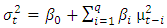(2)

Where

The ARCH (q) model in equation (2) allows for a time-varying variation in conditional variance about previous errors. The unconditional distribution of t in ARCH models is always leptokurtic. The required lag q often turned out to be quite large in applications of the ARCH (q) model. The generalized ARCH (p, q) model (GARCH (p, q)) was developed by Bollerslev (1986) to achieve a more constrained parameterization.

3.2.2. Asymmetric Generalized Autoregressive Conditional Heteroscedasticity (GARCH) Models

In financial markets, if “bad news” has a more pronounced effect on volatility than “good news” of the same magnitude, then a symmetric specification such as GARCH or GARCH-M is not appropriate, since only squared residuals enter the equation, the signs of the residuals or shocks have no effects (in other words, by squaring the lagged error in GARCH, the sign is lost) on conditional volatility. In other word, the model assumes good and bad news have the same effect. However, a stylized fact of financial volatility is that bad news (negative shocks) tends to have a larger impact on volatility than good news (positive shocks). In the case of equity returns, such asymmetries are typically attributed to leverage effects, whereby negative shocks cause the value of the firm to fall which raises the debt-equity ratio thereby increasing the risk of bankruptcy (debt-equity ratios are a key predictor of the probability of default in credit scoring models), (Asemota and Ekejiuba, 2017). This makes shareholders, who bear the residual risk of the firm, to perceive their future cash low stream as being relatively more risky. In order to account for the leverage effects observed in stock returns, the asymmetric models which include: [TGARCH (1,1) and EGARCH(1,1)] are employed.

3.2.3. The Threshold GARCH (TGARCH (1,1)) Model

Asymmetry and leverage (the fact that volatility is negatively correlated with changes in stock returns) are not taken into account by either the ARCH or GARCH models. Although GARCH (p, q) models provide adequate fits for the majority of equity-return dynamics, these models frequently fail to accurately model the volatility of stock returns due to their assumption of a symmetric response between returns and volatility. As a result, the leverage effect of stock returns cannot be taken into account by GARCH models. When it comes to stocks, it is frequently observed that when the market experiences a decline of the same magnitude, volatility is higher than when it experiences a rise of the same magnitude. The threshold GARCH (TGARCH) model was developed by Zakoian (1994) to take into account the existing leverage effect.

The TGARCH model was defined by Zakoian (1994) by permitting the conditional standard deviation to depend on a single lag in innovation. Parameter restrictions that guarantee the conditional variance to be positive are not shown in the specification. However, the TGARCH model's parameters must be restricted and the error distribution chosen to account for stationarity to guarantee stationarity. The GJR-GARCH model is another name for the threshold GARCH model. A straightforward addition to the GARCH model, the GJR model adds a term to account for potential asymmetries.

Using TGARCH (p, q), the following is the generalized specification for the conditional variance:

(3)

Where and 0 if

The condition for non-negativity will be and

In this model, good news implies that and has an impact of and bad news implies that with an impact of . Bad news increases volatility when , which implies the existence of leverage effect in the ith order, and when the news impact is asymmetric. These two shocks of equal size have different effects on the conditional variance.

The first order representation of TGARCH (p, q) is TARCHG (1, 1) given as:

(4)

In this model, good news has a positive impact of and negative news has a negative impact of .

3.2.4. The Exponential GARCH (EGARCH (1,1)) Model

Nelson's (1991) exponential GARCH (EGARCH) model allows for asymmetric effects between asset returns that are positive and negative. Three major shortcomings of the GARCH model were proposed to be addressed by the EGARCH, which takes into account the asymmetric properties of volatility and returns. They are: Restrictions on parameters that guarantee positive conditional variance, insensitivity to volatility's asymmetric response to shock, and difficulty measuring persistence in a strong stationary series.

The EGARCH model's log of the conditional variance indicates that the leverage effect is exponential rather than quadratic. A major advantage of the EGARCH model over the symmetric GARCH model is that it does not restrict the sign of the model parameters because volatility is specified in terms of its logarithmic transformation. As a result, there are no restrictions on the parameters to ensure that the variance is positive. The following is a general description of the EGARCH (p, q) model's conditional variance.

(5)

In this model, good news implies that is positive with total effects and bad news implies is negative with the total effect 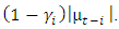When , the expectation is that bad news would have a higher impact on volatility (leverage effect is present) and the news impact is asymmetric if . The EGARCH model achieves covariance stationarity when The EGARCH (1, 1) is specified as:

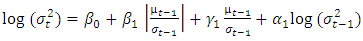(6)

The total effect of good news for EGARCH (1, 1) is and the total effect of bad news for EGARCH is If the null hypothesis that is rejected then, a leverage effect is present, that is, bad news has a stronger effect than good news on the volatility of the stock index return, and the forecasts can be tested by the hypothesis .

3.3. Long Short-Term Memory (LSTM) Deep Learning Model

In this study, LSTMs with better design and gates to control information flow will be used to function as memory units. A typical RNN contains a single hidden state that is updated over time, making it difficult for the network to learn long-term dependencies. The LSTM model addresses this issue by incorporating a memory cell, which is a container capable of storing information for an extended length of time. LSTM architectures can learn long-term dependencies in sequential data, making them ideal for tasks like language translation, speech recognition, and time series forecasting, (Sundermeyer, et al., 2012). In LSTM designs (see Figure 1), the memory cell is controlled by three gates: the input gate, the forget gate, and the output gate. These gates determine what information is added to, removed from, and output from the memory cell. (i) The input gate determines what information is added to the memory cell. (ii) The forget gate determines which information is erased from the memory cell. (iii) The output gate determines what information is output by the memory cell. The LSTM maintains a concealed state that functions as the network's short-term memory. The input layer is represented at the bottom, the output layer is represented at the top and the unfolded recurrent layers are represented horizontally. A unit layer is called a cell that takes external inputs, inputs from the previous time cells in a recurrent framework, produces outputs, and passes information and outputs to the cells ahead in time. The cell state is defined as the information that flows over time in this network (as recurrent connections) with the information content having a value of at time The cell state would be affected by inputs and outputs of the different cells, as we go over the network (or more concretely in time over the temporal sequences). Similarly, the network passes the output y(t) from the previous time to the next time as a recurrent connection, (Kala, 2021).

According to the former settlement, Hochreiter and Schmidhuber (1997) introduced a new architecture: the Long Short-Term Memory (LSTM). This structure works in a similar way of the Elman process, as a matter of fact, it uses one input layer, one hidden layer and one output layer. But the fully self-connected hidden layer presents a complex internal processing unit, named “memory cell”, with a series of corresponding regulators, usually called “gates” that supervise and manage the entering and exiting flow of information. The memory cell, which is depicted in Figure 1, is responsible for keeping note of all the dependencies between inputs. It is usually composed by three gates: a forget gate (𝑓𝑡), an input gate (𝑖𝑡), and an output gate (ℎ𝑡). Each of them, at every time step t, interacts with one element of the input sequence, 𝑥𝑡, and the output of the memory cell from the previous time step, . Specifically, the forget gate defines which information to delete from the cell state, the input gate which data to add to the memory and the output gate which results to use as output from the cell state. Each gate operates similarly to the nodes of the neural network, in fact, they act on the received signals based on the inputs and their weights, and they block or pass the information using an activation function (Fischer & Krauss, 2017). 2017). Figure 2 gives a representation of all the steps in which the work of the memory cell is organised and their explanations from a mathematical point of view. The first step (A) is to decide which information should be delete from the network through the forget gate. So, the activation values 𝑓𝑡 of such gate is calculated and scaled in a range between 0 and 1 by a sigmoid function, meaning respectively “completely forget” or “completely remember”. If the value is a number between them, the information is deleted or kept depending whether the produced value is nearer 0 or 1. The meaning behind the forget gate is ascribable to the fact that, sometimes, the memory cell recognizes as useless, for the assigned task, some collected information and wants to proceed by deleting them. The next step (B) is deciding which data should be added to the network’s cell state, 𝑠𝑡. This operation happens through two phases: the use of a tanh function which designs new candidate variables that could be added to the unit cell and the application of a sigmoid function, which defines the activation values, 𝑖𝑡, of the input gate. In the following step (C), there is the need to update the old state of the memory cell by combining the results of the two previous steps and by transferring them into the cell. The final stage (D) consists in creating results as the output of the memory cell. This concluding step is done, first, through the use of a sigmoid function, that define which data contained in the memory cell should be presented as the output, and then, through the application of tanh function, which delimits the values of the output in a range between -1 and 1 (Olah, 2015).

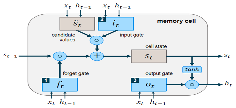Figure 1. Architecture with Long Short-Term Memory (LSTM) Network (Source: Memory Cell in LSTM network (Fischer & Krauss, 2017))

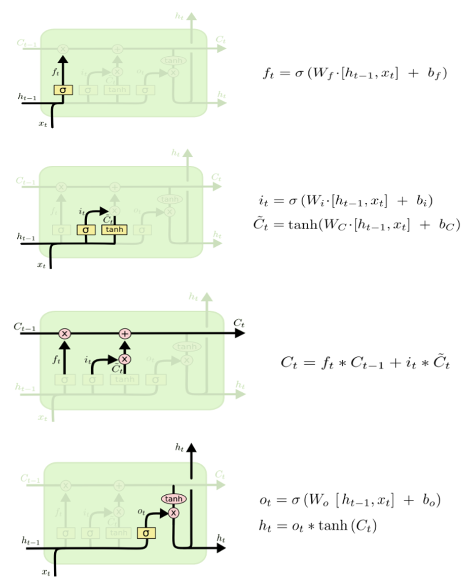Figure 2. Mode of operation of a memory cell in LSTM network (Olah, 2015)

3.4. Model Selection Criteria

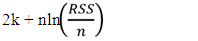
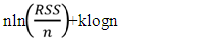
The best model for each of the two Nigeria stock exchange volatility will be selected based on the following criteria; (i) the Akaike information Criterion (AIC), Akaike, H., (1973), (ii) Schwarz information criterion (SIC), Schwarz, G. (1978) and root mean square (RMSE). The volatility of Nigeria stock exchange will based on estimated coefficients of the best conditional variance models, and the model with the least value for these three criteria across the error distributions is adjudged the best fitted. This selection produces the best-fitted conditional variance models for stock returns.

i. The Akaike information criterion (AIC) is:

(7)

ii. Schwarz information criterion (SIC)is:

(8)

iii. The RMSE will produce the preferred model from the two competing models., it is written as;

(9)

4. Result

4.1. Preliminary Result

4.1.1. Descriptive Analysis of Nigeria Stock Exchange Return

Table 1 shows the descriptive statistics of the NSE return series. The average monthly return is 5070.728. The monthly standard deviation is 5707.306, reflecting a high level of volatility in the market. The wide gap between the maximum (20682.29) and minimum (4.82) returns gives support to the high variability of change in the NSE. Under the null hypothesis of normal distribution, Jarque-Bera is zero. The Jarque-Bera value of 56.84852 deviated from normal distribution. Similarly, skewness and kurtosis represent the nature of departure from normality. In a normally distributed series, skewness is 0 and kurtosis is 3. Positive or negative skewness indicate asymmetry in the series and less than or greater than 3 kurtosis coefficient suggest flatness and peakedness respectively, in the returns data. The skewness coefficient of 0.678003 is positively skewed.

Table 1. Descriptive Statistics of Nigeria Stock Exchange Return from 1985-2023

Positive skewness implies that the distribution has a long right tail and a deviation from normality. The empirical distribution of the kurtosis is clearly not normal but peaked.

On the whole, the NSE return series do not conform to normal distribution but display positive skewness and leptokurtic distribution. These results are, however, based on the null hypothesis of normality and provide no information for the parametric distribution of the series.

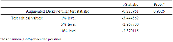
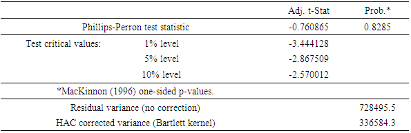
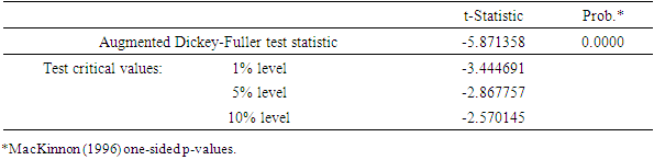
4.1.2. Unit Root Test Results

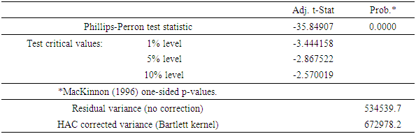
Augumeneted Dicky Fuller and Phillips-Perron unit root test is employed in examining stationarity characteristics of the Nigeria’s stock returns from January 1985 – December 2023. The results of Augumeneted Dicky Fuller and Perron unit root test for data at level and first differenced are presented in Tables 2A-D. The results of Augumeneted Dicky Fuller and Perron unit root test indicates that the market returns are indeed non-stationary. This is shown by the Augumeneted Dicky Fuller and Phillips-Perron test statistics being higher than their corresponding asymptotic critical values at 1% and 5% levels. However, the Phillips-Perron unit root test result of the stock returns show evidence of covariance stationarity as the test statistics are all smaller than their corresponding asymptotic critical values at all the designated test sizes both for constant only and for constant and linear trend. These results confirmed the result observed by visual inspection of time plots reported in Figures 4.

Table 2A. Unit Root test Augumented Dicky Fuller Test (at Level)

Table 2B. Phillips-Perron test statistic (At Level)

Table 2C. Augumented Dicky Fuller Test (at First Difference)

Table 2D. Phillips-Perron test statistic (At First Difference)

4.1.3. Correlogram Test for Heteroskedasticity

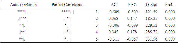
Table 3 presents the Ljung-Box Q-statistics for the heteroskedasticity. It is a test of the null hypothesis that the autocorrelation of the lags are equal to zero. The result indicated that the p-values of the five lags were less than the level of significance, an indication that the model does not exhibits a lack of fit.

Table 3. Correlogram and Ljung-Box Q-statistics Test for Heteroskedasticity

4.1.4. Graphical Presentation of Nigeria Stock Exchange Returns

Figure 3 presents the pattern of level data on return series of the NSE for the period under review, which is January 1985 – December 2023. The level data show that the NSE return series is not stationary indicating the need for differencing. But the return series show sign of returning to its mean suggesting that the series are weakly stationary (See Figures 4). From Figure 5, we see that the NSE stock returns distribution is peaked confirming the evidence of non-normal distribution in Table 1. Peaked distribution is a sign of recurrent wide changes, which is an indication of uncertainty in the return discovery process.

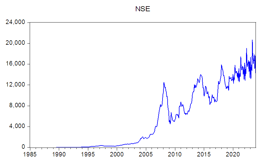Figure 3. Line Graph of Monthly Index for NSE (Jan.1985 – Dec. 2023)

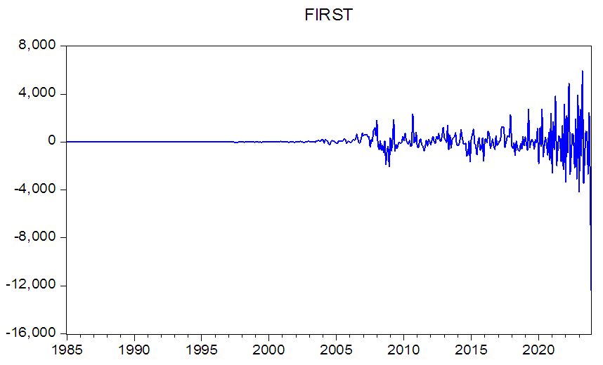Figure 4. Line Graph of Monthly Index of NSE First Differencing (Jan.1985 – Dec. 2023)

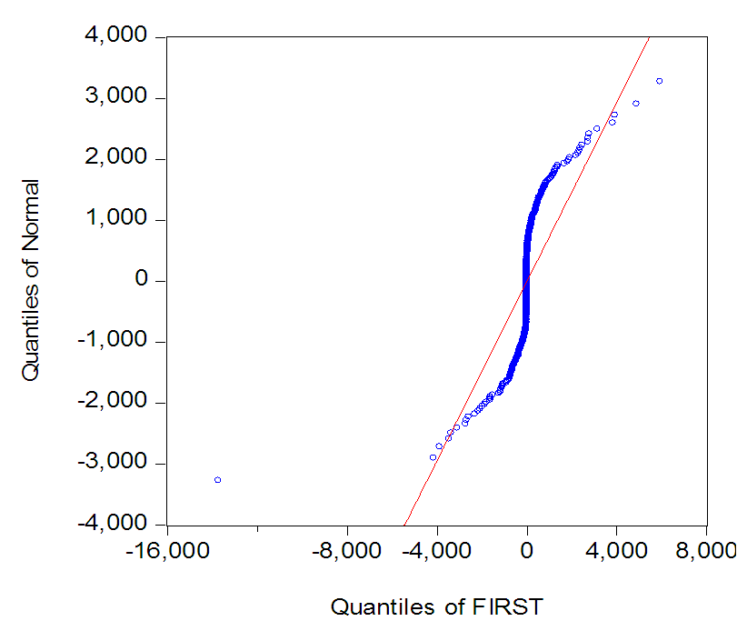Figure 5. Quantile-Quantile Plot for the First Differenced NSE Monthly Returns (Jan. 1985-Dec. 2023)

4.2. ARCH-LM Test for Heteroskedasticity

The result presented in Table 4 indicates result of the residual test of heteroskedasticity for ARCH effects. The test rejects the null hypothesis of no ARCH effects in the residuals of returns. This means that the errors are time varying and can only be modeled using heteroskedastic ARCH family models.

Table 4. ARCH-LM TEST FOR HETEROSKEDASTICITY

4.3. Analysis of Data Using Asymmetric GARCH Type-Models

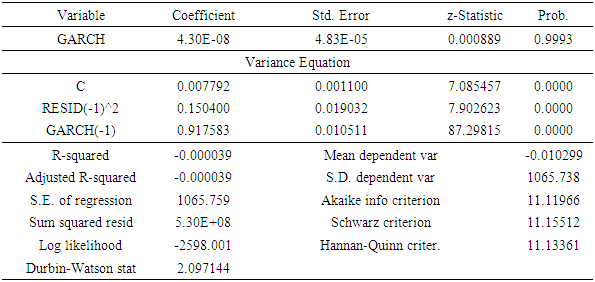
4.3.1. Results of EGARCH (1,1)

The parameter estimates of the asymmetric EGARCH (1, 1) model presented in Table 5 indicates that the coefficient (0.6432) of the ARCH effect is significantly positive at 1% showing that news about previous volatility (past square residual terms) has an explanatory power on current volatility. The GARCH effect coefficient (0.5789) is also significantly positive at 1% level, which shows that past volatility of stock market return is significantly influencing current volatility. The sum of ARCH and GARCH coefficients (1.2221) is a measure of the persistence of variance, and since the value is greater than 1 implies that there is significant high persistence in volatility. As suggested by Engle and Bollerslev (1986), if 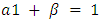, a current shock persists indefinitely in conditioning the future variance. Since the sum of a1 + β represents the change in response function of shocks to volatility persistence, a value greater than unity implies that response function of volatility increases with time and a value less than unity implies that shocks decay with time (Chou, 1988). Therefore, the above result indicates that memory of shocks is remembered in the NSE.

Table 5. EGARCH(1,1) MODEL FOR NSE (1985-2023)

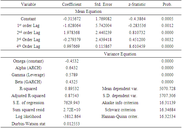
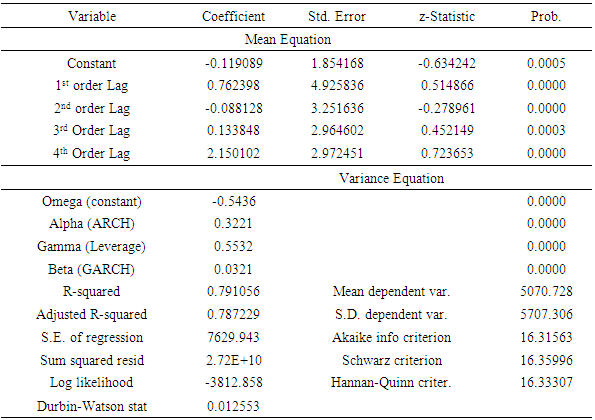
4.3.2. Results of TGARCH (1,1)

The TGARCH (1,1) is an asymmetric model, which is used to investigate the existence of leverage effect in returns of the NSE. The estimates of the model are reported in Table 5. The asymmetric term in the TGARCH (1, 1) model is positive and significant suggesting the existence of leverage effect in returns during the study period. This implies that previous period’s positive and negative shocks have a different effect on the conditional variance.

For the effect of the previous period’s bad news to be greater than the effect of good news of the same magnitude, Gamma should be significant and have a negative sign. On the other hand, for the effect of the previous periods’ positive news to be greater than the effect of bad news of the same magnitude, Gamma should be significant and have a positive sign. Table 6 are the estimates of TGARCH (1,1) model. The asymmetric effect of the TGARCH (1,1), captured by the parameter estimate γ, is positive and significant.

Table 6. TGARCH MODEL FOR NSE (1985-2023)

4.4. Selection of the Best Fitting Asymmetric GARCH Model

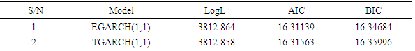
To select the best fitting asymmetric GARCH models with suitable distributional assumption, information criteria such as Akaike information criterion (AIC) due to Akaike (1978) and Schwarz information criterion (SIC) due to Schwarz (1978) are employed in conjunction with log likelihoods (LogL). The best fitting model is one with largest log likelihood and minimum information criteria. Table 7 displays the asymmetric GARCH results of EGARCH (1,1) and TGARCH (1,1) models. The information criteria together with the log likelihood optimally selects asymmetric EGARCH (1,1) as the best candidates to model the stock return volatility in Nigerian stock market.

Table 7. Asymmetric GARCH Model Order Selection

This study compares econometrics models such as GARCH, TARCH, and EGARCH with machine learning techniques such as LSTM. It is necessary to develop a good LSTM model, which significantly depends on the number of layers to be used and the number of nodes present in each layer. Since the LSTM model is compared with GARCH models, to have a fair comparison, the lag order of the ΔVIXt series for the LSTM model is kept the same as that of the GARCH models, i.e., 4. By comparing the AIC and BIC values of training, validation and test data, the number of layers and nodes in each layer of the LSTM was manually determined. The AIC and BIC values for several layer and node combinations and chose the one that performed the best. ReLU activation function is used between the layers, and the optimizer used to minimize the training error is Adam because Adam has been proven to be the best among all the 1st order optimizers available for neural networks (Kandel et al. 2020). Table 8 and 9 present the AIC and BIC performance of the LSTM model using different combinations of layers and nodes, and the best combination for the ΔVIXt series is found to be three LSTM layers with 160, 80, and 5 nodes in each layer, respectively.

Table 8. Comparison of different architectures for the LSTM model with AIC

Table 9. Comparison of Different Architectures for the LSTM Model with BIC

4.5. Comparison of LSTM and GARCH Models Using out of Sample Forecasting Results

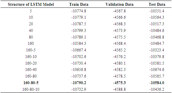
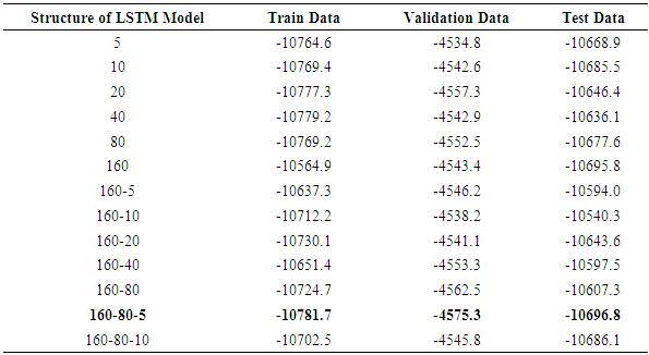
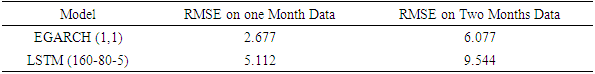
This study compares the performance of the models by forecasting the India VIX volatility from each model for the next two months in the future and then analyzing the results based on three performance metrics, i.e., mean directional accuracy (MDA), mean absolute percentage error (MAPE), and root mean squared error (RMSE). The reason for keeping three performance metrics is to compare the performance of models in different aspects; for example, MDA would tell the performance of models in predicting the direction of volatility, whereas RMSE would explain how far the predictions are from actual values. Table 10 presents the out-of-sample version of models (LSTM and GARCH models) on the MAPE metric in predicting the India VIX values for the next two month.

Table 10. Performance Comparison using RMSE Criterion

5. Discussion of Finding

Overall results from this study provide evidence to show that volatility of stock returns is persistent in Nigeria stock returns data. These results is in tune with the findings from (Enow, 2023) who revealed that stock market volatility will persist at least for some time from the ARCH and GARCH output results. Active traders and market makers need to adapt their strategies in response to the expected volatility persistence. Higher levels of persistence may call for adjustments such as widening stop-loss orders to accommodate larger price swings or using more extended timeframes to capture sustained trends. Portfolio managers may also opt for strategies that thrive in volatile market conditions such as breakout trading or mean reversion strategies. The results also support the evidences of volatility persistence in Nigeria stock exchange as provided by (Godfrey & Agwu, 2018; Ajayi et al., 2019) and existence of leverage effects in Nigeria stock returns provided by Okpara and Nwezeaku (2009), but disagree with their conclusion that stock returns volatility is not quite persistent in Nigeria.

The result of this study also shows that asymmetric EGARCH (1,1) outperformed LSTM model based on the lowest AIC and BIC forecasting accuracy criteria for the Nigerian stock market volatility returns. This result agrees with findings from (Adams and Uchema, 2023) in a study that compared Exponential Generalized Autoregressive Conditional Heteroskedasticity with order p=1 and q= 1, (EGARCH (1,1)) and Recurrent Neural Network (RNN) based on long short term memory (LSTM) model with the combinations of p = 10 and q = 1 layers to model the volatility of Nigerian exchange rates. The results indicated that the Nigeria exchange rate volatility is asymmetric, and leverage effects are evident in the results of the EGARCH (1, 1) model. It was observed also that EGARCH (1,1) performed better than the LSTM model because it provided a smaller MSE values of 224.7, 231.3 and 138.5 for euros, pounds sterling and US Dollars respectively. The study by and The findings of this study is however contradicted by (Chatterjee, et al. (2022) that investigated stock volatility prediction using time series and deep learning methods. The study introduced several volatility models based on the Exponential general autoregressive conditional heteroscedasticity (EGARCH), Glosten-Jagannathan-GARCH (GJR-GARCH), and generalized autoregressive conditional heteroscedasticity (GARCH) frameworks. The three types of GARCH models and the LSTM model were tested for their ability to predict stock volatility in three distinct industries. The findings revealed that the LSTM model performed better in predicting volatility in the pharmaceutical sector than in the banking and IT sectors.

6. Conclusions

This study investigated the volatility of stock market returns in Nigeria using EGARCH (1,1), TGARCH (1,1) and the LSTM models. It also examined asymmetric characteristics in the volatility of the Nigerian stock market returns series from January 1985, to December 2023 and develop a robust forecast model that can properly and timely notify Nigerian stockbrokers of fluctuations in the market. The asymmetric GARCH results of EGARCH (1,1) and TGARCH (1,1) models indicated that asymmetric EGARCH (1,1) is the best candidate model for stock return volatility in Nigerian stock market. The performance of the LSTM model using different combinations of layers and nodes, and the best combination for the ΔVIXt series discovered that three LSTM layers with 160, 80, and 5 nodes in each layer, respectively were the best among the other combinations. The results from EGARCH (1,1) and TGARCH (1,1) models indicated that volatility of stock returns is persistent in Nigeria. The result of the forecasting accuracy of the LSTM and asymmetric GARCHs model based on the Nigerian stock market volatility returns indicated that EGARCH (1,1) outperformed LSTM (160-80-5) model based on the lowest AIC and BIC. EGARCH (1,1) was found to be the appropriate model for forecasting Nigerian stock market volatility returns. Based on the findings of this study, it is recommended that;

(i) Stockbrokers should invest regularly, be consistent in trading, maintain a diversified portfolio and seek professional advice. The strategies will curb the persistent volatility in Nigeria stock return.

(ii) In the comparison between econometric asymmetric GARCH and deep learning’s LSTM, the EGARCH (1, 1) performs better than the LSTM model.

(iii) for modeling and predicting the volatility of Nigeria stock return, EGARCH (1,1) provides the best statistical method.