-
Paper Information
- Paper Submission
-
Journal Information
- About This Journal
- Editorial Board
- Current Issue
- Archive
- Author Guidelines
- Contact Us
American Journal of Mathematics and Statistics
p-ISSN: 2162-948X e-ISSN: 2162-8475
2023; 13(1): 44-59
doi:10.5923/j.ajms.20231301.02
Received: Oct. 6, 2022; Accepted: Oct. 30, 2022; Published: Apr. 15, 2023

Handling Missing Values in Covariate for Modeling Count Data with over Dispersion and Zero Inflation
 Abstract
 Reference
 Full-Text PDF
 Full-text HTML
1Department of Medicine, McMaster University, Hamilton, ON L8N 3Z5 Canada
2Department of Mathematics and Statistics, University of Windsor, Windsor, ON N9B 3P4 Canada
Correspondence to: Rajibul Mian, Department of Medicine, McMaster University, Hamilton, ON L8N 3Z5 Canada.
| Email: |  |
Copyright © 2023 The Author(s). Published by Scientific & Academic Publishing.
This work is licensed under the Creative Commons Attribution International License (CC BY).
http://creativecommons.org/licenses/by/4.0/

The problem of regression analysis of count response data having information on some covariates missing may arise in some practical applications. Further complications, such as, over-dispersion and zero-inflation in the count responses, may also arise. In this paper we develop estimation procedure for the parameters of a zero inflated over/under dispersed count response model in the presence of missing covariates. A zero-inflated negative binomial model with missing covariate information is used. Obtaining maximum likelihood estimates by direct use of the log-likelihood involves multiple numerical integration. To avoid this we develop a weighted expectation maximization algorithm. A simulation study is conducted to investigate the properties of the estimates, in terms of bias, variance, mean squared errors (MSE) and coverage probability (CP). Further simulations are also conducted to study Robustness of the procedure for count data following other over-dispersed models, such as the log-normal mixture of the Poisson distribution. An example and a discussion are given.
Keywords: Count Data, EM Algorithm, Missing Covariate Information, Over dispersion, Regression model, Zero inflation
Cite this paper: Rajibul Mian, Sudhir Paul, Handling Missing Values in Covariate for Modeling Count Data with over Dispersion and Zero Inflation, American Journal of Mathematics and Statistics, Vol. 13 No. 1, 2023, pp. 44-59. doi: 10.5923/j.ajms.20231301.02.
Article Outline
1. Introduction
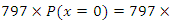
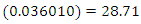
- Discrete data in the form of counts arise in many health science disciplines such as biology and epidemiology. For examples of discrete count data see Deng and Paul (2000, 2005), Bohning, D., Dietz, E., Schlattmann, P., Mendonca, L., and Kirchner, U. (1999), Anscombe (1949); Bliss and Fisher (1953); Bliss and Owen (1958); McCaughran and Arnold (1976); Margolin, Kaplan and Zeiger (1981); Ross and Preece (1985)), Manton, Woodbury and Stallard (1981). The Poisson distribution is the most commonly used distribution for analysing count data. The Poisson distribution has a property that mean and the variance of the distribution are equal to each other. However, in many count data cases this property of the Poisson distribution does not hold, as extra dispersion (variation) is observed in the data, and thus Poisson distribution is not an ideal choice for analysing count data in many applications. The presence of extra dispersion in count data is common in many real life situations. To accommodate this extra dispersion situation in count data a well known model is the negative binomial distribution, which is very convenient and common in practice. For the applications of the negative binomial distribution see for example Engel (1984); Breslow (1984); Margolin et al. (1989); Lawless (1987); Manton et al. (1981). The negative binomial distribution has flexibility in its parameterization and has been used differently by different authors. For example, see Paul and Plackett (1978); Barnwal and Paul (1988); Paul and Banerjee (1998); Piegorsch (1990), Deng and Paul (2000, 2005). Often times a particular count (for example zero) may arise in the data more than the expected number. Count data with many zeros may not be explained properly by a model such as a Poisson distribution and a negative binomial distribution, so a zero inflated Poisson distribution and a zero inflated negative binomial distribution can be the ideal choice. For example see Deng and Paul (2000, 2005), Ridout, Demetrio and Hinde (1998), Williamson, Lin, Lyles and Hightower (2007). Count data in the presence of both extra dispersion as well as zero inflation can be analysed by a zero inflated negative binomial model. Extensive work has been done to fit zero-inflated and over-dispersed count data model to real life data. For example, see Ridout, Demetrio and Hinde (1998), Hinde and Demetrio (1998), Li, Lu, Park, Kim, Brinkley and Peterson (1999), Hall (2000), Lee, Wang and Yau (2001), Wang, Lee, Yau and Carrivick (2003), Lord, Washington and Ivan (2005), Jiang and Paul (2009), Cameron and Trivedi (2013). Also a lot of work has been done to test the presence of zero-inflation and/or over-dispersion. For example, see Mullahy (1997), Dean (1992), Greene (1994), Broek (1995), Deng and Paul (2000), Xie, He, and Goh (2001), Paul, Jiang, Rai and Balasooriya (2004), Williamson, Lin, Lyles and Hightower (2007).An example of count data in the presence of both extra dispersion as well as zero inflation can be found in Bohning, Dietz, Schlattmann, Mendonca, and Kirchner (1999). Bohning et al. (1999) present a set of data on a prospective study of dental status represented by decayed, missing and filled teeth (DMFT) index of school children from an urban area of Belo Horizonte (Brazil). DMFT index scores can range from 0 to 28 or 32 per individual. The tooth is considered as decayed, when a carious lesion or both carious lesion and a restoration are present. The tooth is considered as missing if the tooth has been extracted due to caries. If a temporary or permanent filling is present in the tooth, or the filling of the tooth is defective but not decayed, then the tooth is considered as a filled tooth. The total number of tooth of a person having these properties would be the DMFT index for the person. More details of DMFT index can be found in Cappelli and Mobley (2007). The DMFT index was observed for 797 children at the beginning and at the end of the study. For the purpose of illustration here we consider DMFT index observed at the beginning of the study which, when summarized in terms of index and its frequency, are (index, frequency): (0,172), (1,73), (2,96), (3,80), (4,95), (5,83), (6,85), (7,65), (8,48). The mean and the variance of these counts are 3.3237 and 6.6387, which show over-dispersion in the data. Further, the observed frequency of zeros is 172 as opposed to the expected frequency of
 showing that the data are also zero-inflated under a Poisson model.Regression analysis of count data may be further complicated by the existence of missing values either in the response variable and/or in the explanatory variables (covariates). Extensive work has been done on regression analysis of continuous response data with some missing covariates under normality assumption. See, for example, Rubin (1977), Little and Rubin (1987, 2002, 2014), Lipsitz and Ibrahim (1996), Ibrahim, Chen and Lipsitz (1999), Ibrahim, Chen, Lipsitz and Herring (2005), Sinha and Maiti (2007), Maiti and Pradhan (2009).Some work on missing values has also been done on logistic regression analysis of binary data. See, for example, Ibrahim (1990), Lipsitz and Ibrahim (1996), Ibrahim and Lipsitz (1996), Ibrahim, Chen and Lipsitz (1999), Ibrahim, Chen and Lipsitz (2001), Sinha and Maiti (2007), Maiti and Pradhan (2009).Rubin (1977) and Little and Rubin (1987, 2002, 2014) discuss various missingness mechanisms. If the missingness does not depend on observed data, then the missing data are called missing completely at random (MCAR). If the missing data mechanism depends only on observed data, then the data are missing at random (MAR). The MAR is also known as ignorable missing That is, in this case, the missing data mechanism is ignored. If the missing data mechanism depends on both observed and unobserved data, that is, failure to observe a value depends on the value that would have been observed, then the data are said to be missing not at random (MNAR) in which case the missingness is nonignorable. For more detailed discussion on missing data mechanism see Ibrahim et al. (2005).The purpose of this paper is to develop estimation procedure for the parameters of a zero-inflated negative binomial (ZINB) model for count data when information on some covariates on some individuals are missing.The problem of missing responses in ZINB model was dealt earlier by the same researchers in Mian and Paul (2016); and guided to this research.Obtaining maximum likelihood estimates by direct use of the log-likelihood involves multiple numerical integration. To avoid this we develop a weighted expectation maximization algorithm following Ibrahim (1990). A simulation study is conducted to investigate the properties of the estimates, in terms of bias, variance, mean squared errors (MSE) and coverage probability (CP). Further simulations are also conducted to study Robustness of the procedure for count data following other over-dispersed models, such as the log-normal mixture of the Poisson distribution. The method is illustrated using the dental epidemiology data of Bohning et al. (1999) discussed above.The procedure for the estimation of the parameters are developed in Section 2. Results of a simulation study is reported in Section 3. The illustrative example is given in Section 4 and a discussion leading to some conclusions is given in Section 5.
2. Estimation in Zero-Inflated and Over-Dispersed Count Data Regression Model with Missing Values in the Explanatory Variables
2.1. The ZINB Model
- The zero-inflated negative binomial regression model (Deng and Paul, 2005) can be written as
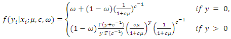 | (1) |
 and
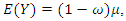
and  where
where  is the zero-inflation parameter. We denote this distribution by
  distribution.Suppose that data for the
  of n subjects are
  which are realizations from
  where
where  represents the response variable and
  represents a
  vector of covariates with the regression parameter
 such that
  Here
Here  is the intercept parameter in which case
  for all
2.2. Estimation of the Parameters with no Missing Values in Covariate
- For complete data the likelihood function is
 | (2) |
 the log likelihood, apart from a constant, can be written as
  | (3) |
 can be estimated by directly maximizing the loglikelihood function (2.3) or by simultaneously solving the estimating equations Given in Appendix A.
2.3. Estimation of the Parameters with Missing Values in Covariate
2.3.1. Estimation under MCAR
- In case of MCAR, missingness of the data do not depend on observed data and the subjects having the missing observations are deleted before the analysis. For estimation procedure the likelihood function remains same an given in equation (2.3) with reduced sample size having only complete observations.
2.3.2. Estimation under MAR
- As some of the observations in some covariates (on some individuals) may be missing we write
 (the
(the  covariate value of the
  individual)
  | (4) |
 given in equation (1), the log-likelihood of
  is
is 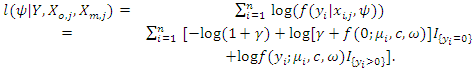 | (5) |
 and
and  the observed and the missing values for the
  covariate are involved in
  In MAR, conditional probability of missing covariate values depends on observed values
  Parameters of the missingness mechanism are completely separate and distinct from the parameters of the model (1). In likelihood based estimation considering MAR, missingness mechanism can be ignored from the likelihood and missing data (covariate) that are missing at random are often known as ignorable missing, but the subjects having these missing covariates can not be deleted before the analysis. (see Little and Rubin, 1987, 2002, 2014 and Ibrahim, Chen, Lipsitz and Herring, 2005 for detailed discussion).Following Ibrahim (1990), and Lipsitz and Ibrahim (1996), we consider covariates
  are random variables with finite parameters
  These covariates
  have distribution that can be expressed by one dimensional conditional distribution as
  where
where  more specifically
 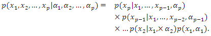 | (6) |
 have some missing observations and these missing observations are missing at random. For this covariate
  the probability of observing the missing observations (conditional on the response, y and the other completely observed covariates) does not depend on the missing covariate itself and any other covariate with unobserved observations, but may depend on the response as well as completely observed covariate. This flexible characteristics of MAR comes to an aid during estimation. Only if this probability of observing the missing observations depend on the response as well as completely observed covariate, then
  needs to incorporate in the main likelihood
  . Note that in practical regression problem, the covariates are usually very poorly dependent among each other, otherwise multicollinearity problems can be solved by using other statistical tools.To incorporate this covariate distribution with the complete data loglikelihood of
  following Ibrahim (1990), we specify the joint distribution of
  by using the conditional distribution of
  and the marginal distribution of
  that is
  . Following Ibrahim (1990) we consider,
  are independent and
  are independently
  and identically distributed for all
  observations. Considering this, our likelihood becomes
  | (7) |
 and the covariates model
  are separate as well as distinct. This idea facilitates the separate maximization of the both parts of the likelihood. Moreover, covariates
  can be discrete or continuous or mixture of discrete and continuous. All the covariates in
  may not have missing observations, in that case, distributions of the completely observed covariates can be ignored (detailed discussion on this are available in Lipsitz and Ibrahim (1996), and Ibrahim et al. (2005)).In this scenario, our main goal is to estimate the parameters of the count data model
  by maximizing the following loglikelihood (Little and Rubin, 1987, 2002, 2014 p.89) with respect to the parameters
 | (8) |
 | (9) |
 is not, in general, straight forward. However, the EM algorithm (Dempster, Larid and Rubin, 1977) is a very useful tool for obtaining maximum likelihood estimates with missing observations.The EM algorithm uses two iterative steps known as the expectation-step (E-step) and the maximization-step (M-step). Following Little and Rubin (1987, 2002, 2014), the E-step provides the conditional expectation of the log-likelihood
  given the observed data
  and current estimate of the parameters
  Suppose we have a covariate with missing observations and
  of the
  observations of the covariate are observed and
  observations are missing and
  be an arbitrary number of iterations during maximization of the log-likelihood, then the E-step of the EM algorithm for the
  observation of the missing covariate for
  iteration can be written as
  | (10) |
 become
  | (11) |
 iteration is
  | (12) |
 become
  | (13) |
 is the conditional distribution of the missing covariate given the observed data and the current
  estimate of
  However, in many situations,
  may not always be available. Following Ibrahim, Chen, Lipsitz and Herring, 2005 and Sahu and Roberts, 1999, we can write
 where
where  is the complete data distribution given in (1),
  is the distribution for the covariates where the missing values exist and both have very elegant forms. For the
  of the B missing observations of the covariate we take a sample
  from
from  using Gibbs sampler (see Casella and George, 1992 for details). Then, following Ibrahim, Chen and Lipsitz (1999) and Ibrahim, Chen, Lipsitz and Herring (2005)
  can be written as
  | (14) |
 is maximized. Here maximizing
  is analogous to maximization of complete data log likelihood where each incomplete covariate being replaced by
  weighted observations. More details of EM algorithm by method of weights can be found in Ibrahim, 1990; Lipsitz and Ibrahim, 1996(a,b), Ibrahim, Chen and Lipsitz, 1999, 2001; Ibrahim, Chen, Lipsitz and Herring, 2005; Sinha and Maiti, 2007; Maiti and Pradhan, 2009.Variance covariance matrix of the estimates of the parameters is calculated by inverting the observed information matrix at convergence (Efron and Hinkley, 1978) which is
  | (15) |
 above are given in the Appendix.
2.3.3. Estimation under MNAR
- If missing observation in the covariate are considered to be missing not at random (MNAR), the missingness depends on the values that would have been observed. In this case, probability of missing observations in covariate depends on the observed values of the other covariate, response and the values of the covariate that would have been observed. This missing data mechanism cannot be ignored and needs to be incorporated in the likelihood. The missing observations that follow this missing data mechanism are known as nonignorable missing. To incorporate this missing data mechanism in the data likelihood, it is natural to specify a parametric model for this mechanism. Let
 be a random vector of missingness indicator for the
  covariate.
  | (16) |

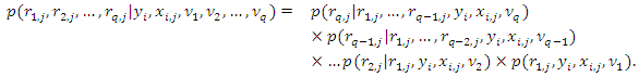 | (17) |
 are the indexing parameters for the conditional distribution of
  Highest value for
  can be
  Logistic regression is a popular choice for the one dimensional distribution for
 | (18) |
 Note that choice of variables for the model of
  is important. Often many variables in this model are not necessarily significant, and more importantly parameters in the model for
  are not the primary interest for estimation. Detailed discussion on this can be found in Ibrahim, Lipsitz and Chen (1999) and Ibrahim, Chen and Lipsitz (2001).Following Ibrahim, Lipsitz and Chen (1999), after incorporating the model for missingness mechanism
  the data loglikelihood become
  | (19) |
3. Simulation Study
- A simulation study was conducted to investigate the properties of the estimates, in terms of bias, variance, mean squared errors (MSE) and coverage probability (CP) of estimates. We use data under four scenarios: (i) data are observed completely, (ii) some observations in covariates are missing completely at random (MCAR), (iii) some observations in covariates are missing at random (MAR), and (iv) some observations in covariates are missing not at random (MNAR). Simulations are conducted for continuous as well as discrete covariate.Responses are generated from the zero-inflated negative binomial model (1) with
 where
where 
 and
and  Note that
  is the intercept parameter, hence
  The explanatory variable
  was generated from
  when covariate is considered to be continuous, and from
  in case of discrete covariate. We consider 5%, 10% and 25% missing observations in the explanatory variable. For empirical coverage probability we take nominal level
  Simulation results for continuous covariate are given in Table 1 whereas results for discrete covariate are in Table 2.
 | Table 1. Properties (estimate, bias, variance, mse, coverage probability (cp)) of the estimates of the parameters, data simulated from NB  based on 5000 simulation runs (continuous covariate) based on 5000 simulation runs (continuous covariate) |
 | Table 2. Properties (estimate, bias, variance, mse, coverage probability (cp)) of the estimates of the parameters, data simulated from NB  based on 5000 simulation runs (discrete covariate) based on 5000 simulation runs (discrete covariate) |
 distribution. In order to see whether similar properties of the estimates hold when over-dispersed data are generated from another distribution rather than the
  distribution. Such a distribution that has been used earlier by others (Lawless, 1987 and Paul and Banergee, 1998) is the log-normal
  mixture of the Poisson distribution with
 and
and  , where
  and
and  are the parameters of the
  . In the situation in which there are covariates we take
  . For more details of generating data from the log-normal mixture of the Poisson distribution see Lawless (1987).The parameter values used to simulate data from the zero-inflated log-normal mixture of the Poisson distribution were the same as those used to generate data from the zero-inflated negative binomial distribution. We also used the same percentages of missing data as those in the previous case.Results of the simulation study of the zero-inflated log-normal mixture of the Poisson distributed data are given in Table 3 and Table 4. Fortunately, we arrived at very similar conclusions of the results given in Table 1 and Table 2. This shows, perhaps, that the results will remain similar irrespective of the mechanism in which over-dispersed count data are generated.
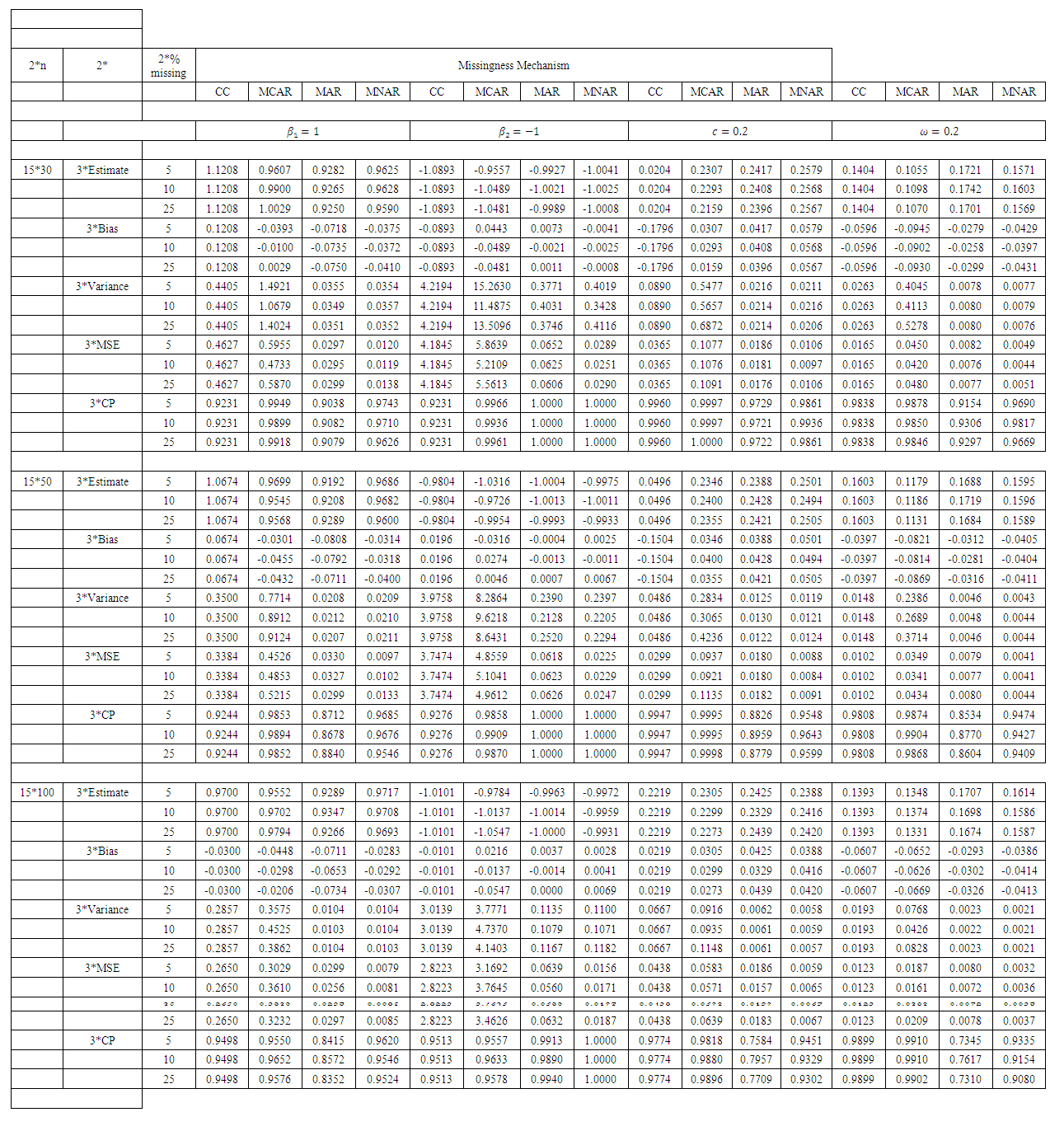 | Table 3. Properties (estimate, bias, variance, mse, coverage probability (cp)) of the estimates of the parameters, data simulated from lognormal mixture of Poisson  based on 5000 simulation runs (continuous covariate) based on 5000 simulation runs (continuous covariate) |
 | Table 4. Properties (estimate, bias, variance, mse, coverage probability (cp)) of the estimates of the parameters, data simulated from lognormal mixture of Poisson  based on 5000 simulation runs (discrete covariate) based on 5000 simulation runs (discrete covariate) |
4. An Illustrative Example
- We now analyze a set of data from a prospective study of dental status of school children from Bohning et al. (1999). The children were all 7 years of age at the beginning of the study. Dental status were measured by the decayed, missing and filled teeth (DMFT) index. Only the eight deciduous molars were considered so the smallest possible value of the DMFT index is 0 and the largest is 8. The prospective study was for a period of two years. The DMFT index was obtained at the beginning of the study and also at the end of the study.The data also involved 3 categorical covariates: gender having two categories (0 - female, 1 - male), ethnic group having three categories (1 - dark, 2 - white, 3 - black) and school having six categories (1 - oral health education, 2 - all four methods together, 3 - control school (no prevention measure), 4 - enrichment of the school diet with ricebran, 5 - mouthrinse with 0.2% NaF-solution, 6 - oral hygiene).For the purpose illustration of our method we deal with the DMFT index data obtained at the beginning of the study (as in Deng and Paul, 2005). The DMFT index data at the beginning of the study are: (index, frequency): (0,172), (1,73), (2,96), (3,80), (4,95), (5,83), (6,85), (7,65), (8,48). We then fitted a zero-inflated negative binomial model to the complete data and data with missing observations in covariate. To obtain data with missing observations in covariate we randomly deleted a certain percentage (5%, 10%, 25%) of the observed covariate gender. The model fitted was


 , where
  represents the intercept parameter and
  represents the regression parameter for gender,
  and
and  represent the regression parameters for the ethnic groups 1 and 2, and
  and
and  represent the regression parameters for school 1, school 2, school 3, school 4, and school 5 respectively.The estimates of the mean parameter
  where
where 
 the over dispersion parameter
  and the zero inflation parameter
  based on the zero-inflated negative binomial model, under different percentages of missingness, and their corresponding standard errors are presented in Table 5. It is to note that the estimates of the parameters
  and
and  and the corresponding standard errors changes with the amount of missingness in the covariate (this is expected as it depends on which observations have remained in the final data set). In general, the standard errors of the estimates are larger than those under complete data. However, estimates of
  do not vary much irrespective of the percentage missing and the missing data mechanism. The same comment applies to
  although for
  is a bit higher under MNAR.
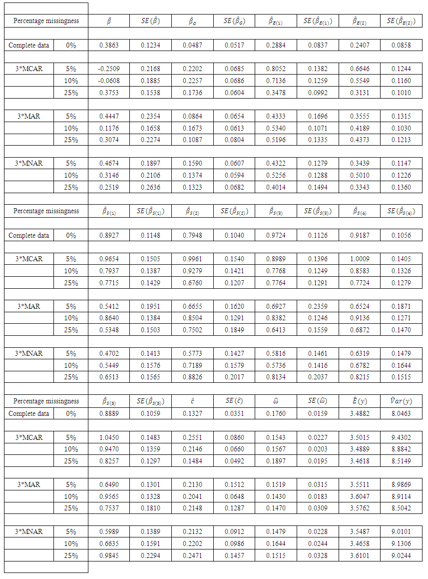 | Table 5. Estimates and Standard Errors of the parameters for DMFT data with covariates |
5. Discussion
- We have developed estimation procedure for the parameters of a zero inflated negative binomial model in presence of missing observations in covariate. We applied a weighted expectation- maximization algorithm (Ibrahim, 1990) for the maximum likelihood estimation of the parameters. Although missing data methodologies have been developed extensively in literature, the current development for the estimation of the parameters of a zero inflated negative binomial model in presence of missing covariate is new.The overall message of the simulation study is that estimation procedure performs in a stabilized fashion irrespective of the missingness mechanism and percentage of missing observation though the performance is relatively noticeable for the smaller sample size.
6. Appendix
6.1. Appendix A: Estimating Equations for the Parameters  in the Model (2.3)
 | (20) |
 | (21) |
 | (22) |
6.2. Appendix B: The Gibb Sampler
- To use the Gibbs sampler we need to generate each sample point of
 by using Gibbs sequence. For example Gibbs sequence for
  is
is  For large
  According to Sahu and Roberts (1999)
  can be considered as a block and can obtained from
  In this scenario, for each missing response, samples are considered as a block. For example if there are 5 missing response, then there are 5 blocks. Sahu and Roberts (1999) also mentioned that most practical cases, missing observations are independent of parameters and considers as a single block. In this case, 5 missing observations can be treated as a single block. In our model, missing responses are independent of parameters and hence we follow Sahu and Roberts (1999) for Gibbs sampling. We stop the sequence and obtain the required sample for which the absolute deviation of parameters between two consecutive steps become minimal. Extensive explanation of Gibbs sampler are available in Casella and George (1992) and Sahu and Roberts (1999).
Appendix C: Elements of the Observed Information Matrix
- From equation (14) we have
 | (23) |
 is analogous to maximization of complete data log likelihood,
  in (3) where each incomplete response being replaced by
  weighted observations. The elements of the observed information matrix are as given below.
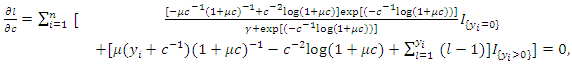
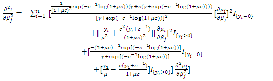 | (24) |
 | (25) |
 | (26) |
 | (27) |
 | (28) |
 | (29) |
 | (30) |
ACKNOWLEDGEMENTS
- This research was partially supported by the Natural Science and Engineering Research Council of Canada.