-
Paper Information
- Paper Submission
-
Journal Information
- About This Journal
- Editorial Board
- Current Issue
- Archive
- Author Guidelines
- Contact Us
American Journal of Mathematics and Statistics
p-ISSN: 2162-948X e-ISSN: 2162-8475
2023; 13(1): 1-43
doi:10.5923/j.ajms.20231301.01
Received: Sep. 25, 2022; Accepted: Nov. 13, 2022; Published: Mar. 15, 2023

Approximating Non-Asymptoticalness, Skew Heteroscedascity and Geo-spatiotemporal Multicollinearity in Posterior Probabilities in Bayesian Eigenvector Eigen-Geospace for Optimizing Hierarchical Diffusion-Oriented COVID-19 Random Effect Specifications Geosampled in Uganda
 Abstract
 Reference
 Full-Text PDF
 Full-text HTML
Benjamin G. Jacob 1, Ricardo Izureta 1, 2, Jesse Bell 1, Jeegan Parikh 1, Denis Loum 3, Jesse Casonova 4, Tracy Gates 1, Kayleigh Murray 1, Leomar White 1, Jane Ruth Aceng 5
1College of Public Health, University of South Florida, Tampa, USA
2One Health Group, Universidad de las Americas
3Nwoya District Local Government, Nwoya, Uganda
4Health International Program
5Uganda Ministry of Health, Kampala, Uganda
Correspondence to: Benjamin G. Jacob , College of Public Health, University of South Florida, Tampa, USA.
| Email: |  |
Copyright © 2023 The Author(s). Published by Scientific & Academic Publishing.
This work is licensed under the Creative Commons Attribution International License (CC BY).
http://creativecommons.org/licenses/by/4.0/

This paper presents two space-time model specifications, one based upon the generalized linear mixed model (GLMM), and the other upon Moran eigenvector space-time filters. We identify optimization algorithms to fit a COVID-19 regression model to a training dataset. of non-asymptotical, multicollinear, skew heteroscedastic, estimator and other non-normalities due to violations of regression assumptions We did so to learn more about how regression functions can characterize geo-spatiotemporally, spilled over, hierarchical diffusion of the viral infection in Uganda at the sub-county district-level. Our objective was to predictively prioritize and target, hyper/hypo-endemic transmission variables. A Moran spatial filtering technique was employed which performed an eigenfunction, second order, eigen-spatial filter eigendecomposition of the random effects (REs) in varying, temporally dependent, georeferenced, diagnostically stratified, clinical, environmental, and socio-economic, endemic, transmission-oriented determinants which rendered (SSRE) and spatially unstructured (SURE) components. The RE model incorporated synthetic eigen-orthogonal eigenvectors derived from a geographic connectivity matrix to account for SSRE and SURE in standardized z scores stratified by multi-month, viral, infection yield, due to geo-spatiotemporal, spill-over, hierarchical diffusion of the virus at the sub-county, district-level. We calculated the conditional probabilities and derived the conditional distribution functions for the regressed diagnostic determinants including the probability density function, the cumulative density function, and quantile function. A Poisson random variable mean response specification was written as follows:  where esitk and eHith respectively were the ith elements of the K < NT and H < NT selected eigenvectors and Estk and EHth were extractable from the doubly-centered space-time
  and
and 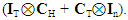 The expectation attached to the equation, i.e., RE ≡ SURE was satisfied, with both having trivial SSRE components. In the Bayesian context, the SSRE component was modelled with a conditional autoregressive specification which captured residual, zero autocorrelation (i.e., geographic chaos), non-homoscedastic, asymptotical non-normality and multicollinearity in the georeferenced, aggregation/non-aggregation-oriented, COVID-19, specified, diagnostically stratified, prognosticator, clustering propensities. The model’s variance implied a substantial variability in the prevalence of COVID-19 across districts due to the hierarchical diffusion of the virus. Site-specific, semi-parametric eigendecomposable, eigen-orthogonal, eigen-spatial filters are useful in revealing the influence of non-normality [e.g., heterogeneity of variances] in diagnostic, COVID-19 variables due to violations of regression assumption and hence are more accurate in prediction of georeferenceable, hyper/hypo-endemic, sub-county, transmission-oriented district-level geolocations compared with a global model in which the non-homogenous erroneous estimators and their evidential uncertainty-oriented probabilities do not vary across Bayesian eigenvector eigen-geospace.
Keywords: COVID-19, Hierarchical diffusion, Moran eigenvector, Bayesian, Eigen-spatial-time filtering, Uganda
Cite this paper: Benjamin G. Jacob , Ricardo Izureta , Jesse Bell , Jeegan Parikh , Denis Loum , Jesse Casonova , Tracy Gates , Kayleigh Murray , Leomar White , Jane Ruth Aceng , Approximating Non-Asymptoticalness, Skew Heteroscedascity and Geo-spatiotemporal Multicollinearity in Posterior Probabilities in Bayesian Eigenvector Eigen-Geospace for Optimizing Hierarchical Diffusion-Oriented COVID-19 Random Effect Specifications Geosampled in Uganda, American Journal of Mathematics and Statistics, Vol. 13 No. 1, 2023, pp. 1-43. doi: 10.5923/j.ajms.20231301.01.
Article Outline
1. Introduction
- In recent studies Farzanegan et. al. (2020) (Farzanegan et. al., 2020) revealed globalization to be positively linked to the reported numbers of COVID-19 cases in that more globalized countries experience higher exposure to outbreaks (Zimmermann et. al., 2020) as do ‘global cities’ within countries (Ali and Keil 2006). On a global scale, Sirkeci and Yüceşahin (2020) suggest that the spread of COVID-19 in China follows a relocation diffusion pattern, while Kuebart and Stabler (2020) observe relocation diffusion of COVID-19 in Germany based on existing interpersonal networks. Internationally, globalization supports relocation diffusion, as public health studies have repeatedly acknowledged (e.g., Tatem and Rogers 2006). COVID-19 has rapidly spread via international air travel (Candido et al. 2020) connecting countries with high levels of tourism and trade (Ribeiro et al. 2020). Another study Farzanegan et. al (2020) found that almost all KOF (Swiss Economic Institute) globalization sub-indices (Gygli et al. 2019) exhibit a robust positive association with the number of district-level, COVID-19, reported cases, with social globalization—which proxies migration and civil rights among other measures—being the most important predictor both in magnitude and statistical significance.Another mode of spatial diffusion of COVID-19 is through geographic, spatiotemporal, (henceforth geo-spatiotemporal), hierarchical diffusion, which characterizes spread from large settlements to smaller ones, or from more internationally significant cities (e.g., ‘global city-regions’) to those less significant. In the case of COVID-19 previous research suggests that large metropolitan areas experience greater spread due to the larger number of people, their closer proximity and increased movement. For example, Ali et al. (2020) observed, spilled over, geo-spatiotemporal, hierarchical diffusion of COVID-19 from the largest cities to smaller settlements in Brazil. Similarly, Sirkeci and Yüceşahin (2020) observed hierarchical diffusion of COVID-19 infection in countries including the United States, the United Kingdom, South Korea and Italy among others.Certain settlement characteristics are associated with hyper/hypo-endemic, geo-spatiotemporal, geosampled, hierarchical, diffusion-related, aggregation / non-aggregation-oriented, parameterizable, estimator tendencies of an infectious, viral, disease process, including diagnostically stratifiable, determinants associated with the level of urbanization, population density and transportation network and accessibility. Larger and denser cities have been shown to increase vulnerability to viral, infectious disease spread (Connolly et. al. 2021) by creating the requisite preconditions for higher numbers of human interactions wherein higher densities act to increase the intensity of such interactions. Tarwater et. al. (2001) and Andersen et. al., (2021) find that urbanization is a significant forecaster of COVID-19 transmission within the United States, while Carozzi (2020) finds urban density to be a explanatory, (i.e., statistically significant), linearizable, regression, district-level, subcounty-level determinant of the pandemic.Additionally, there are marked differences in population characteristics—population size, development levels, household size and age structure—and environmental co-factors affecting the diffusion of a viral infectious disease. Recent research regarding COVID-19 has identified multiple environmental co-factors associated with this incident, such as, temperature (Liu et al., 2020; Wang et al., 2020; Zhu and Xie, 2020), air pollution (Wu et al., 2020), and humidity (Auler et al., 2020; Gupta et al., 2020). Further types of behaviour such as smoking (Taghizadeh-Hesary aghizadeh-Hesary 2020) WaSH effects (Das et al., 2020) and socio-economic vulnerability (Kang et al., 2020) may regulate the severity and rate of COVID-19 spread due to district-level, geo-spatiotemporal, hierarchical diffusion of the virus. These diagnostic, geossmpled, clinical, environmental, and socio-economic determinants may be evaluated in a regression framework for optimally, prognosticating, hyper/hypo-endemic geolocations. In so doing resources and other prevention measures (targeting and prioritizing vaccine distribution) may be correctly allocated to specific sub-county district-level regions.Multiple linear regression is a statistical method which has been employed to understand the relationship between multiple predictor variables and a response variable (district-level COVID-19 prevalence) for modelling determinants associated to hierarchical diffusion of the SARS-CoV-2 virus If the X (independent variable), or Y (dependent variable) from which the COVID 19 data to be analyzed by linear regression were sampled, violate one or more of the linear regression assumptions, the results of the analysis may be incorrect or misleading. For example, if the assumption of independence is violated, in a COVID-19 model then linear regression may not be appropriate for modelling variables associated to the pandemic. If the assumption of normality is violated, or outliers are present in the model outcome, then the linear regression goodness of fit test may not be the most powerful or informative test available, and this could mean the difference between detecting a linear fit or not in these models. A nonparametric, robust, or resistant regression method, a transformation, a weighted least squares linear regression, or a nonlinear model may result in a better fit. If the population variance for Y is not constant in a linear COVID-19 model, a weighted least squares linear regression, or a transformation of Y may provide a means of fitting a regression adjusted for the inequality of the variances. Often, the impact of an assumption violation on the linear regression result depends on the extent of the violation (such as the how inconstant the variance of Y is, or how skewed the Y population distribution is) (Hosmer and Lemeshew 2002). Some small violations in a prognosticative, hyper/hypo-endemic, hierarchical, diffusion-related, diagnostically stratified, COVID-19 regression model may have little practical effect on the analysis, while other violations may render the linear result uselessly incorrect or uninterpretable. Problem associated to violations of regression assumptions in a prognosticative, hierarchical, diffusion -related, COVID-19 model (skew heteroscedasticity, multicollinearity) may be solved in a principled, time series, dependent, inferential, Bayesian framework for learning aggregation / non-aggregation-oriented, hyper/hypo- endemic, model, selection sites, and density estimation. Bayesian statistics is a theory in the field of statistics based on the Bayesian interpretation of probability where probability expresses a degree of belief in an event. The degree of belief may be based on prior knowledge about the event, such as the results of previous experiments, or on personal beliefs about the event. (district COVID-19 transmission). This differs from several other interpretations of probability, such as the frequentist interpretation that views probability as the limit of the relative frequency of an event after many trials.Precision forecast maps targeting and prioritizing hyper/hypo-endemic, transmission-oriented, diagnostically stratifiable, COVID-19 determinants associated with a subcounty, district-level, transmission-related, hot /cold spot requires disturbance-free regressors. (e.g., non-Gaussianity of the errors) for asymptotically optimally reflecting the geo-spatiotemporal, hierarchical, diffusion-related dissemination of the sampled determinants. Statistical error or uncertainty is the amount by which an observation differs from its expected value (Freedman 2008), the latter being based on the entire population from which the statistical unit was chosen randomly. The expected value, being the mean of the entire population, may be typically unobservable in an empirical, non-asymptotical, vulnerability-oriented, geo-spatiotemporally dependent, district-level, COVID-19, hierarchical diffusion-related, subcounty, prognosticative model, and hence the statistical error may not be observable. A residual (or fitting deviation), on the other hand, is an observable estimate of the unobservable statistical error, which may have embedded in noisy non-normal trajectories in empirically regressed georeferenced datasets of district-level, sub-county, COVID-19, diagnostic, stratifiable, geo-spatiotemporal, hierarchical, diffusion-related, vulnerability-oriented, estimated parameterizable determinants. In regression analysis, the distinction between errors and residuals is subtle and leads to the concept of studentized residuals (i.e., the quotient resulting from the division of a residual by an estimate of its standard deviation). Commonly in the literature, public health, epidemiological, viral, infection, transmission-related, predictive, risk models (e.g., hyper/hypo-endemic, hierarchical, diffusion, COVID-19, regression paradigm) are constructed in the form of a Student’s t-statistic, with the estimate of error varying between sentinel site, time series, dependent, geosampled, data, capture points (e.g., district level, aggregation / non-aggregation-oriented, diagnostic determinants). Given an unobservable function that relates the independent variable to the dependent variable, the deviations of the dependent variable observations [e.g., scaled-up, subcounty, district-level prevalence] from this function would be the unobservable errors in an epidemiological, hierarchical, diffusion-related, COVID-19, stratified, predictive, risk model. If one runs a regression on some data, then the deviations of the dependent variable observations from the fitted function are the residuals (Hosmer and Lemeshew 2002). Optimally, if the linear COVID-19 model is applicable, a scatterplot of residuals plotted against an independent variable (e.g., number of inmates with positive clinical presentation in a sub-county local jailhouse) in an epidemiological, district-level, hierarchical, diffusion- related, prognosticative, regression model, the renderings should be random about zero with no trend to the residuals. If the geosampled data (e.g., temporally dependent, georeferenced, clinical, environmental, and or, socio-economic, diagnostic, stratified, empirical, COVID-19, hierarchical, diffusion estimators) exhibit a trend in regression space then the model is likely erroneous, for example, the true function m a quadratic or higher order polynomial. If they are random, or have no trend, they will exhibit heteroscedasticity. Homoscedasticity, or homogeneity of variances, is an assumption of equal or similar variances in distinct groups being compared. (Hosmer and Lemeshew 2002). This is an important assumption of parametric statistical tests because they are sensitive to any dissimilarities. Uneven variances in samples [e.g., heteroscedasticity] in empirical, regressed, geosampled, datasets of epidemiological, district-level, hyper/hypo-endemic, geo-spatiotemporal, COVID-19, sub-county, georeferenceable, aggregation / non-aggregation-oriented, diagnostic estimators will result in inaccurate, model, test results. For example, assuming a clinician or researcher constructs a mean ordinary least squares (OLS) regression for optimizing targeting and prioritizing an empirical geosampled dataset of hierarchical, diffusion-related, diagnostic determinants of COVID-19. This model would assume nothing about the shape of the dependent or independent variable; it would make only assumptions about the distribution of the errors as measured by the residuals. When these assumptions are violated, the results of the regression may be wrong. The relationship between "extent of violation" and "type of error" in an epidemiological, district-level, subcounty, vulnerability-oriented, regression, COVID-19, model output for targeting and prioritizing, aggregation / non-aggregation-oriented, hyper/hypo-endemic, transmission, due to hierarchical diffusion of the virus has not been contributed to the literature.The mean squared error [MSE] of a regression is a number computed from the sum of squares of the computed residuals, and not of the unobservable errors (Freedman 2008). If that sum of squares in an epidemiological, COVID-19, diagnostic, stratified, regression, prognosticative model is divided by n, the number of geosampled observations [i.e., subcounty, hyper/hypo-endemic, hot/cold spot, hierarchical, diffusion-oriented, risk-related, aggregation / non-aggregation-oriented determinants], the result is the mean of the squared residuals. Since this would be a biased estimate of the variance of the unobserved errors in the viral, infection, prognosticative, epidemiological, risk model, the bias could be removable by dividing the sum of the squared residuals by df = n − p − 1, instead of n, where df is the number of degrees of freedom (n minus the number of parameters (excluding the intercept) p being estimated - 1). This would form an unbiased estimate of the variance of the unobserved errors and the MSE rendered by the epidemiological, hierarchical, diffusion, forecast-related, vulnerability-oriented, diagnostic, COVID-19, district-level, subcounty, stratified, model output.Another method to calculate the MSE in an epidemiological, prognosticative, subcounty, district-level, scaled-up, prognosticative, hierarchical, diffusion-related, diagnostically stratified, COVID-19, vulnerability-oriented model for optimizing targeting and prioritizing, potential, hyper/hypo-endemic determinants is by analysing the variance of linear regression employing a technique like that used in ANOVA (they are the same as ANOVA is a type of regression). In these paradigms the sum of squares of the residuals (aka sum of squares of the error) is divided by the df (which would be equal to n − p − 1, where p is the number of, diagnostic, sampled, COVID-19, stratified, clinical, socioeconomic and or environmental parameters for example, estimated in the model (one for each variable in the regression equation, not including the intercept). An infectious disease modeller or research collaborator may also calculate the mean square of the sampled, district-level, hierarchical, diffusion-related, subcounty, aggregation / non-aggregation-oriented, COVID-19, stratified, vulnerability-oriented, model estimators by dividing the sum of squares of the model minus the df which would be just the number of selected diagnostic parameters (i.e., clinical, environmental and/or socioeconomic determinants). Subsequently the F value can be calculated for the model by dividing the mean square of the derived output by the mean square of the error, and then determining significance (which is why one needs to calculate the mean squares to begin with) in an epidemiological, COVID-19, district-level, subcounty, prognosticative, vulnerability-related model. An F-test is any statistical test in which the test statistic has an F-distribution under the null hypothesis (Hosmer and Lemeshew, 2002).Hence, to compare residuals from an epidemiological, hierarchical, diffusion-related, hyper/hypo-endemic, COVID 19, risk model at different inputs, a viral infectious disease modeller or researcher would need to adjust the residuals by the expected variability of residuals, (i.e., studentizing). In statistics, studentization is the adjustment consisting of division of a first-degree statistic derived from by a sample-based estimate of a population standard deviation (Hosmer and Lemeshew 2002). This is particularly important in the case of detecting outliers, where the case in question is somehow different than the others in an epidemiological, COVID-18, estimator dataset. For example, a large residual may be expected in the middle of the domain in an empirical, hierarchical, diffusion-related, district-level, COVID-19, aggregation/non-aggregation-oriented, hyper / hypo-endemic, vulnerability, model output for targeting and prioritizing, subcounty, hot/cold spot, diagnostic determinants, but considered an outlier at the end of the domain. Outlier detection algorithms are intimately connected with robust statistics that down-weight some observations to zero especially in epidemiological, viral, infection forecast-oriented, vulnerability models (e.g., Jacob et al. 2014). In this experiment we define several outlier detection algorithms related to an empirical epidemiological dataset of georeferenced, geosampled, hierarchical, diffusion-related, sub-county, district-level, hyper/hypo-endemic, COVID-19, stratified, risk, model estimators. Next, we apply asymptotic theory for evaluating the predictors. In statistics, asymptotic theory, or large sample theory, is a framework for assessing properties of estimators and statistical tests. (Estrada and Kanwal, 2002). Within this framework, it is often assumed that the sample size n may grow indefinitely; the properties of estimators and tests are then evaluatable under the limit of n → ∞. Subsequently, a COVID-19 modeller, researcher or data analyst may investigate the gauge, [i.e., the fraction of wrongly detected disturbances] in the model and establish asymptotic normality and Poissonian theory for the gauge. In probability theory and statistics, the Poisson distribution is a discrete probability distribution that expresses the probability of a given number of events occurring in a fixed interval of time or space if these events occur with a known constant mean rate and independently of the time since the last event (Haight 1967). We employed the Poisson distribution to estimate how many times a district-level, COVID-19, hierarchical, diffusion, transmission-related, event was likely to occur within "X" periods of time at a sub-county in Uganda. Poisson distributions are used when the variable of interest is a discrete count variable (Haight 1967). Finally, we eigendecompose the COVID-19 estimators and then determined robustness of the georeferenced, determinants in Bayesian eigenvector eigen-geospace.Eigen-spatial filters are used to decompose a matrix into eigenvectors and eigenvalues which are eventually applied in methods used in machine learning, such as in the Principal Component Analysis method or PCA [Griffith 2003]. Our assumption was that an eigendecomposed, asymptotic estimator model may optimize predictively targeting and prioritizing, hierarchical, diffusion-related, hyper / hypo-endemic, subcounty, district-level, transmission-related geolocations by generating error-free time series, dependent, epidemiological determinants. Asymptotic regression is appropriate when a contiguous region on the right or left (or both) of the input is expected to deviate systematically from the regression model in a finite fashion. Such regions ("non-asymptotic regions") often occur in time series dependent, vulnerability-oriented, viral infection, risk, model analysis (Jacob et al. 2013, Griffith 2006). We assumed that the local asymptotic normality property may be establishable for an epidemiological, district-level, diagnostically stratifiable, georeferenced, hierarchical, diffusion-related, COVID-19, parameter estimator, predictive, vulnerability-oriented, regression model for optimizing targeting and prioritizing, subcounty, hyper/hypo-endemic, transmission sites with fractional ARIMA p, d, q errors. ARIMA is an acronym for “autoregressive integrated moving average” which is a model used in statistics and econometrics to measure events that happen over a period. The model is used to understand past data or predict future data in a series. We assumed that the results from such a paradigm would allow for solving, in an asymptotically optimal way, a variety of inference problems such as hypothesis testing, discriminant uncertainty analysis, rank based testing, etc. for constructing an epidemiological, geo-spatiotemporal, vulnerability-related, COVID-19, diagnostic, stratified, model for optimizing predictively targeting and prioritizing, georeferenceable, aggregation / non-aggregation-oriented, hyper/hypo-endemic, subcounty, district-level hierarchical, diffusion-related determinants. Further, we assumed that the problem of testing linear constraints on the parameters could be treated in some detail in an asymptotic regression equation for generating robust, (i.e., noiseless) iterative, interpolative estimators of COVID-19. In this experiment we also wanted to deal with the problem of extracting statistically significant determinants associated to geolocations of georeferenced subcounty epicentres of hyper/hypo-endemic, COVID-19, transmission at the district level in the presence of nuisance parameters. Nuisance parameters occur when reality and data are complex enough to require models with multiple parameters, but inferential interest is confined to a reduced set of parameters. Making inferences on geosampled, hierarchical, diffusion-oriented, transmission-related estimators in a prognosticative, vulnerability-oriented, geo-spatiotemporal, COVID-19, epidemiological, subcounty, scaled up, district-level, model output that are not influenced by the nuisance parameters is difficult. Marginal or conditional likelihoods may be pertinent for quantifying nuisance parameters. These are proper likelihoods so all the likelihood ratio based evidential techniques may be employable for unbiasing the estimator non-normality in the regression model. Output. Unfortunately, marginal, and conditional likelihoods are not always obtainable. Royall (2000) recommends the use of profile likelihood ratio as a general solution. According to Royall, the profile likelihood ratio is an ad hoc solution as true likelihoods are not being compared. Nevertheless, he finds the performance of the profile likelihood ratio to be very satisfactory for prognosticative modelling. Likelihood ratio tests are standard statistical tools used to perform tests of hypotheses. The null distribution of the likelihood ratio test statistic is often assumed to be χ2, following Wilks’ theorem. In statistics Wilks' theorem (Wilks 1938), offers an asymptotic distribution of the log-likelihood ratio statistic which may be usable to produce confidence intervals [CIs] for maximum likelihood (ML) estimates, or as a test statistic for performing the likelihood-ratio test in, for example, an epidemiological, geo-spatiotemporal, subcounty, district-level, hierarchical, diffusion-related, prognosticative, COVID-19, vulnerability model, regression estimation. Statistical tests (such as hypothesis testing) require knowledge of the probability distribution of the test statistic. This is often a problem for likelihood ratios, especially in an epidemiological, COVID-19, prognosticative, risk model where the probability distribution can be exceedingly difficult to determine. Suppose that the dimension of Ω=v is related to the dimension of Θ0=r. Under regularity conditions and assuming H0 is true, the distribution of Λn would tend to a chi-squared distribution with df equal to v−r as the sample size tends to infinity. With this theorem in hand (and for n large), we can compare the value of our log-likelihood ratio to the expected values from a χ2v−r distribution. However, in many circumstances relevant to an epidemiological, prognosticative, hierarchical, diffusion-related, sub-county, district-level, COVID19, diagnostic, stratified, vulnerability-related model this theorem may not be applicable.In this contribution we reveal practical ways to identify erroneous variable situations due to violations of regression assumptions and provide guidelines on how to construct valid inference for statistically forecasting COVID-19 endemic, district-level transmission due to hierarchical diffusion of the virus in Uganda. In our expanded view of evidence, the profile likelihood ratio may not be ad hoc as the profile likelihood ratio may be shown to be an evidence function in an epidemiological, hierarchical, diffusion-related, vulnerability-oriented, COVID-19, diagnostically stratified, parameter estimation, district-level, subcounty, geo-spatiotemporal, forecast model. We show that the probability of misleading evidence from a profile likelihood ratio is not constrained by the universal bound, and can exceed 1/k. Thus, even in this first expansion of the concept of evidence from the likelihood ratio of two simple hypotheses, it may be that ML may be decoupled from the likelihood ratio in an epidemiological, COVID 19, stratified, prognosticative, hierarchical, diffusion-related, risk-related paradigm. In so doing, non-normal information (e.g., multicollinear, uncertainty estimators) may be optimally extractable prior to mapping the forecasted, georeferenced, hot/cold spot, aggregation/non-aggregation, district-level, transmission-oriented, subcounty epicentres of COVID-19 transmission. In this experiment, we assumed that a regression, may be able to model the roles of scaled up georeferenced, subcounty, human settlement, and population characteristics employing socio-economic determinants, for example, of reported COVID-19 hierarchical diffusion in a Generalized Linear Mixed Model (GLMM). Operationally GLMMs estimate fixed and random effect (REs) and are especially useful when the dependent variable is binary, ordinal, count, or quantitative but not normally distributed. In statistics, a RE model, also called a variance components model, is a statistical model where the model parameters are random variables (Diggle et. al. 2002). It is a kind of hierarchical linear model which assumes that the data being analysed are drawn from a hierarchy of different populations whose differences relate to that hierarchy. A RE model is a a mixed model here the model parameters are random variables. (Hosmer and Lemeshew 2002).A mixed model, mixed-effects model or mixed error-component model is a statistical model containing both fixed effects and REs. These models are useful in a wide variety of disciplines in the physical, biological and social sciences. They are particularly useful in settings where repeated measurements are made on the same statistical units (longitudinal study), or where measurements are made on clusters of related statistical units. Because of their advantage in dealing with missing values, mixed effects models are often preferred over more traditional approaches such as repeated measures analysis of variance for uncertainty-oriented, error, parameter, estimator quantification.Further, GLMMs can model autocorrelation. Spatial autocorrelation is the correlation among values of a single variable strictly attributable to their relatively close locational positions on a two-dimensional surface, introducing a deviation from the independent observations assumption of classical statistic (Griffith 2003). Random effects (REs) may be described as inference predictor variables about the distribution of values (e.g., quantifiable variance amongst diagnostically stratifiable, hierarchical, diffusion-related, semi-parameterizable, time series, dependent, COVID-19, regression, estimator values of the response at different measurable levels (e.g., time series, zero autocorrelation to non-zero autocorrelation). In fixed-effects models (e.g., regression, ANOVA), there is only one source of random variability. This source of variance is the random sample one may employ to measure for example, empirically geosampled, geo-spatiotemporally scaled-up, district-level, georeferenceable, aggregation / non-aggregation-oriented, hyper/hypo-endemic, subcounty, COVID-19, diagnostic determinants. Capturing the precise variability across individuals’ “residual” variance (in linear models, this is the estimate of σ2 or MSE) is vital for optimal forecasting capability (Freedman 2008). Mixed effects models—whether linear or generalized linear—are different in that there is more than one source of random variability in the data. We may account for these differences in an epidemiological, hierarchical, diffusion-related, COVID-19, district-level, prognosticative, vulnerability model for geo-spatiotemporally targeting georeferenceable, subcounty, hyper/hypo-endemic, hot/cold spot, endemic, transmission zones through the incorporation of REs. Further, quantifiable random intercepts may allow the outcome to be higher or lower for each regression-related, explanative, predictor variable (e.g., a hyper/hypo-endemic, subcounty, district-level, geosampled, hierarchical, diffusion-related, COVID-19, diagnostically stratifiable, clinical, environmental, or socioeconomic determinant). A random intercept model estimates separate intercepts for each unit of each level at which the intercept is permitted to vary. This is one kind of RE model. Another RE model includes random slopes, and estimates separate slopes (i.e., coefficients, betas, effects, etc.Random slopes may allow the fixed effects to vary for each geosampled variable in a hierarchical diffusion-related, forecast-oriented, COVID-19, regression model. The slope is interpreted as the change of Y for a one unit increase in X (Hosmer and Lemeshew 2002). This is the same idea for the interpretation of the slope of the regression line. β ^ 1 which may represent the estimated increase in Y per unit increase in X in an epidemiological, COVID-19, regression, risk, model estimation. Note that the increase may be negative. Regression may also model the relationship between a set of hierarchical diffusion-related geosampled, COVID-19 predictor (independent) variables and specific percentiles (or "quantiles") of a target (dependent) variable, which may be the median. This may be calculable as the square of the correlation between the observed Y diagnostic values and the predicted Y values using the estimators for constructing the viral infection, risk model. The output may reveal stratifiable, time series, dependent, diagnostic determinants associated to hyper/hypo-endemic, transmission-related, COVID-19, hot/cold spot, subcounty district-level geolocations. Alternatively, the method of least squares is about estimating uncertainty parameters by minimizing the squared discrepancies between observed data, and their expected outcome. Here we employed the least square method in the context of a regression problem, where the variation in one geosampled, diagnostic, stratified, hierarchical, diffusion-oriented prognosticator [i.e., the response variable Y] was partly explained by the variation in the other variables, [i.e., clinical, socio-economic, and environmental, COVID-19 sampled co-variables X]. For example, the variation in the subcounty, district-level model results Y here was caused by variation in abilities and diligence X of the sampled time series variation on the scaled-up prevalence Y which was primarily due to variations in socioeconomic, environmental, and clinical conditions X. Given the value of X, the best prediction of Y (in terms of MSE) in the model was the mean f (X) of Y given X in the model renderings. The function f (i.e., the regression function) was estimated from sampling n co-variables and their responses (x1, y1), . . . , (xn, yn). whereas the method of least squares estimates the conditional mean of the response variable across sampled data capture points, (e.g., subcounty, district-level, COVID-19, stratified, hierarchical, diffusion-related, explicatory, predictor, variable, discrete integers). Quantile regression estimates the conditional median of the response variable (Rao 1972).Quantile regression is an extension of linear regression that could be usable when the conditions of linear regression are not met (i.e., linearity, homoscedasticity, independence), for example, in an epidemiological, diagnostically stratified, COVID-19, hierarchical, diffusion-related, vulnerability-oriented, prognosticative, model, empirical, sample dataset for optimizing multicollinear, non-asymptotical, diagnostic determinants. We assumed that optimizing the geosampled epidemiological data would enable robustly predictively, targeting and prioritizing, district-level, subcounty, aggregation / non-aggregation-oriented, hyper/hypo-endemic, hot/cold spot, transmission-related zones employing multiple varying, georeferenced, clinical, socio-economic, and environmental, diagnostic, stratified determinants.It is already observed that time series, dependent, regressable, diagnostic determinants of poor demographic, socio-economic, built environment and poor health structure are elucidative co-factors in hierarchical, diffusion-related, forecast models for regressively targeting georeferenceable, district-level, subcounty, (e.g., zip code), geospatial, hot/cold spots, or endemic transmission for infectious diseases like, tuberculosis, (Jacob et. al. 2014) and HIV, (Khalatbari-Soltani et al. 2020) Influenza Bluhm and Pinkovskiy (2020) and pneumonia (Bärnighausen et al. 2020; Huang et al. 2017, Farr et al. 2000). These studies suggest that similar patterns might be visible for this emerged virus. However, more, time series, sensitive, regression modelling studies are warranted that consider a large variety of epidemiological, aggregation/non-aggregation-oriented, hyper/hypo-endemic, COVID-19, diagnostically stratified, georeferenceable, determinants for optimizing predictive mapping subcounty, district-level, spill-over, geo-spatiotemporal, hierarchical diffusion of the virus in developing countries. In so doing, potential intervention geolocations (district-level, subcounty transmission-related geolocations) may be regressively detected Moreover, most of the current contributions in the literature do not emphasize quantitating non-normality in time series, dependent, hierarchical, diffusion-oriented, forecast, regression-related, epidemiological COVID-19 model, diagnostic co-factors (i.e., clinical, environmental, socioeconomic determinants ) which need to be explored to gain more awareness about this pandemic from a district-level, geo-spatiotemporal, hyper/hypo-endemic, hot/cold spot, predictive, cartographic perspective. Hence, the main question that arises in this experiment is can we accurately regressively forecast, spill-over, geo-spatiotemporal, hierarchical diffusion of the COVID-19 virus in Uganda at the subcounty district-level employing linear/non-linear regressable, diagnostically stratified, environmental, socio-economic, and clinical, diagnostic determinants? Importantly, if any regression assumptions is violated in an epidemiological, multivariate, geosampled, hierarchical, diffusion-oriented, COVID-19, risk model for targeting sub-county, district-level, hyper/hypo-endemic transmission epicentres [e.g., if there are nonlinear relationships between dependent and independent variables), then the forecasts, [i.e., statistically significant (i.e., R square >90%), diagnostic, determinants targeting a hot spot], CIs), and scientific insights yielded, [e.g. causation covariates of the stratified, hierarchical diffusion] may be (at best) inefficient or (at worst) seriously biased (skew non-homoscedastic}, or misleading [non-elucidative, erroneous predictor]. In statistics, OLS are a type of linear least squares method for estimating the unknown parameters in a linear regression model. OLS chooses the parameters of a linear function of a set of explanatory variables by the principle of least squares: minimizing the sum of the squares of the differences between the observed dependent variable [values of the district-level, hierarchical-diffusion-related, hyper / hypo-endemic, time series, dependent, potentially forecastable COVID-19, estimator variable being observed) in an epidemiological, empirical, georeferenced dataset of stratifiable, subcounty, regressed, diagnostic determinants], for example, and those predicted by the linear function of the independent variable. Geometrically, this would be seen as the sum of the squared distances, parallel to the axis of the dependent variable, between each sample, data, capture point in the dataset and the corresponding point on the regression surface—the smaller the error the better the model fits the data. The resulting estimator may be expressible by a simple formula, especially in the case of a linear regression, hierarchical, diffusion-related, prognosticative, COVID-19, stratified, diagnostic, parameterizable estimator model in which there is a single regressor (i.e., geosampled hot/cold spot determinant) on the right side of the regression equation. The OLS estimator is consistent when the regressors are exogenous, and—by the Gauss–Markov theorem—optimal in the class of linear unbiased estimators when the errors are homoscedastic and serially uncorrelated. Under these conditions, the method of OLS provides minimum-variance mean-unbiased estimation when the errors have finite variances. Under the additional assumption that the errors are normally distributed, OLS would be the ML estimator. However, while having a highly skewed dependent variable in an epidemiological, hierarchical, diffusion-related, district-level, vulnerability model for optimizing targeting and prioritization of aggregation/non-aggregation-oriented, COVID-19-related, hot/cold spot, subcounty, transmission-oriented determinants does not violate an assumption, it may make OLS regression rather inappropriate. OLS regression models the mean, and the mean is (usually) not a good measure of central tendency in a skewed distribution (Hosmer and Lemshew 2002). The median may be modelled with regression. In addition, when the dependent variable (e.g., district-level, COVID-19 prevalence) is highly skewed the interest may be in modelling the tails of the distribution.Ideally the statistical software employed to construct an epidemiological, COVID-19, prognosticative, risk model for prioritizing and targeting, hyper/hypo-endemic, district-level, transmission-related geolocations should automatically provide charts and statistics that test whether regression assumptions are satisfied. Unfortunately, software packages do not provide such output by default (additional menu commands must be executed or code must be written) and some (such as Excel’s built-in regression add-in) offer only limited options. RegressIt does provide such output and in graphic detail. However, there are many examples in the literature of outputs from models constructed in RegressIt that violates all regression assumptions [e.g., multivariate normality, no multicollinearity, no zero autocorrelation, non-Gaussian non-asymptoticalness]. These regression prognosticative models are likely to be accepted by a naïve user based on a large value of the R-square. An example of an epidemiological, vulnerability-oriented, geo-spatiotemporal, prognosticative, hierarchical, diffusion-related, diagnostically stratifiable, COVID-19, vulnerability model that may satisfy regression assumptions reasonably well, may be obtainable from a nonlinear transformation of the geosampled diagnostic determinants. The normal quantile plots from these models may reveal the correct geo-spatiotemporality of hierarchical, diffusion-related, explicatory predictors which may be measureable for revealing an actual representative of a hyper/hypo-endemic, infected, georeferenced, hot/cold spot-related, COVID-19, district-level, subcounty population. The quantile-quantile (q-q) plot is a graphical technique for determining if two empirical sampled datasets come from populations with a common distribution (Cressie 1993). These are important considerations in any form of statistical modelling of time series, dependent, COVID-19, stratifiable, hierarchical, diffusion-related, diagnostic determinants although they do not refer to properties of the linear regression equation per se. Spatial statistics (e.g., variogram clouds Moran scatterplots, eigenvector spatial filters) and GIS mapping may aid the process of providing insights to fight against a pandemic and improving public health by identifying outliers in geo-spatiotemporal, subcounty, district-level, COVID-19, sample, parameterizable, regression, estimator datasets. For example, the Spatial Statistics toolbox in ArcGIS ProTM contains statistical tools for analyzing spatial distributions, patterns, processes, and relationships in various geospace. Doing so may enable unbiasing, spatial error non-normality asymptotically by quantitating multicollinear, zero autocorrelatable skew, heteroscedastic, non-exploratory estimators in an empirical dataset of eigendecomposable, geosampled, subcounty, district-level, georeferenced, aggregation/non-aggregation-oriented, geo-spatiotemporal, hierarchical, diffusion-related, COVID-19, diagnostically stratifiable, epidemiological, hot/cold spot, risk, model, eigen-spatial filter, eigen-orthogonal synthetic eigenvectors.Eigenvectors are a special set of vectors associated with a linear system of equations (i.e., a matrix equation) that are sometimes also known as characteristic vectors, proper vectors, or latent vectors (Marcus and Minc 1988). While there may be similarities between spatial and nonspatial (traditional) statistics in terms of concepts and objectives, spatial filtering statistics are unique in that they were developed specifically for use with geographic data. Unlike traditional non-spatial statistical methods, they incorporate space (proximity, area, connectivity, and/or other spatial relationships) directly into their mathematics.Our assumption in this experiment was that the Spatial Statistics toolbox could determine overarching directional trend in an eigenfunction, geo-spatiotemporal, eigen-decomposed dataset of grid-stratifiable, eigen-spatial filter, geosampled, COVID-19, hierarchical, diffusion-oriented, district-level, subcounty, diagnostic determinants. In so doing we would be able to identify geo-statistically significant, hyper/hypo-endemic, georeferenceable, hot spot/cold spot, clustering spatial outliers by teasing out variables associated to violations of regression assumptions. We wanted to assess overall patterns of clustering, or dispersion, group attribute features based on ArcGIS ProTM geolocation, land cover classification (e.g., sub-county, peri-urban, agro-ecosystem, rural pastureland, riverine tributary, an urban low income residential neighbourhood etc.) employing regressively predictable, geosampled, geo-spatiotemporal, district-level, hierarchical, diffusion-related, spill-over, COVID-19, diagnostically stratifiable, aggregation/non-aggregation-oriented, hyper/ hypo-endemic, covariate, feature, attribute similarities, (e.g., georeferenced, sub-county, hot/cold spot, cluster with homogenous tribal economy) for exploring appropriate scale of analysis, and non-normal variability in estimator relationships in Bayesian eigenvector eigen-geospace. The workflow involved multiple steps to progress from pre-processing to segmentation, training sample selection, classifying, and assessing accuracy. Each step was iterative, and the process required in-depth knowledge of the input classification schema, classification methods, expected results and acceptable accuracy. Infectious diseases diffuse over space and time through inherently heterogeneous, geographical processes (Hufnagel 2004). The geographical concept of diffusion may be defined as the spread of a phenomenon across space of which disease diffusion through interpersonal transmission is but one variant (Dalvi et al. 2019). Here, we investigated the role of globalization, settlement, and population heterogeneous characteristics amongst geosampled, multivariate, aggregation / non-aggregation- oriented, diagnostic determinants of reported, COVID-19-related, geo-spatiotemporal, hierarchical diffusion between subcounties and districts in Uganda as an outcome of transmission between individuals. Although each new case is a product of interpersonal transmission—both directly via contact, and indirectly via fomites— one of our hypotheses in this experiment was that COVID-19 hierarchical, diffusion can occur across large, subcounty, district-level distances as an outcome of human movement and mobility. Understandings of viral transmission lie more firmly within the academic domain of virology than diffusion does, which is a fundamentally geographic phenomenon that can be applicable to other forms of spread [for example, innovation diffusion (Hägerstrand 1967)]. Different underlying non-linear, exploratory, epidemiological, empirical processes (e.g., spline back-fitted kernel smoothing of additive auto-regressors of geosampled, time series, dependent, diagnostic, stratified, clinical, socio-economic, or environmental determinants) may describe types of geo-spatiotemporal hierarchical diffusion of COVID 19 at the subcounty, district-level. Expansion diffusion identifies the general tendency for phenomena to spread ‘outward’ and infectious diseases are most associated with contagious (expansion) related diffusion, indicating potential direct transmission between georeferenced neighbours in a particular geolocation (e.g., urban park night club, sports bar primary or secondary school, church, local fish market etc.) due to their physical proximity (Golub 1993).In this experiment, varying, time series, district-level, risk-related, stratified, COVID-19, hierarchical, diffusion-oriented, diagnostic determinants of georeferenceable, sub-county, district-level, transmission-related, hot/cold spots, were mapped in ArcGIS Pro 2.9 and other software packages to examine the COVID-19 situation in Uganda. This study in Uganda with respect to COVID-19, we assumed could be helpful in (i) accessing the role of different influencing epidemiological, regression model, multivariate, diagnostic co-factors [e.g., non-normally distributed, heterogeneity in variance estimates derived from regressed, time series, dependent, geo-spatiotemporally, diagnostically stratifiable, hierarchical, diffusion-oriented, georeferenced, clinical, environmental and socioeconomic determinants], to the practitioners and administrators; (ii) addressing the spatial vulnerability of the community to the COVID-19 district-wide [e.g., provide fully Bayesian intrinsic, autoregressive priors models delineating subcounty, georeferenceable, hot /cold spot geolocations of hyper/hypo-endemic transmission]; and, (iii) development of effective mitigation strategies.Moran's Indices (I) statistics were employed in the analyses to estimate latent, non-zero, global, spatiotemporal autocorrelation and spatial distribution of the georeferenced, district-level, subcounty, COVID-19 cases employing the multivariate, geosampled, hierarchical, diffusion-oriented, clinical, socioeconomic, and environmental, time series, dependent, diagnostically, stratified determinants. Moran's I is a measure of geospatial autocorrelation which is characterizable by a correlation in a signal among nearby georeferenced locations in eigenvector eigen-geospace (Griffith 2003). Geo-spatiotemporal autocorrelation exists because real world phenomena are typified by orderliness, pattern, and systematic concentration, rather than randomness. Tobler’s First Law of geography encapsulates this situation: "everything is related to everything else, but near things are more related than distant things." To this maximum should be added the qualifier: “but not necessarily through the same mechanisms.” In other words, autocorrelation means a dependency exists between georeferenced time series, epidemiological, sampled, data capture points [i.e., re-infection cases in an hyper/hypo-endemic, transmission-oriented, COVID-19, diagnostically stratifiable, subcounty, district-level, hot spot] based on an empirical dataset of geosampled, geo-spatiotemporal, hierarchical, diffusion-related, georeferenced, regression-oriented, prognosticative, diagnostic determinants [e.g., a socioeconomic index such as high human household count in a low income, urban commercial neighbourhood] in proximal geolocations. Autocorrelation can also occur as a systematic pattern in values of other exogenous observational predictors across geolocations on a georeferenced district map due to underlying common co-factors [e.g., high disease transmission infection rate in a zip code, geospatial cluster]. Latent geo-spatiotemporal autocorrelation is more complex than one-dimensional (d) autocorrelation since spatial correlation is multi-dimensional (i.e., 2 or 3 dimensions of space) and multi-directional. Our assumption was that Moran's I may help to optimize [i.e., remove residual, non-normal, multicollinear and/or skew heteroscedastic, zero autocorrelated, non-asymptotical parameters) in an eigendecomposed, georeferenced, geo-spatiotemporal, empirical, sampled dataset of subcounty, district-level, hierarchical, diffusion-related, hyper/hypo-endemic, COVID-19, diagnostically stratified, transmission-oriented determinants] and their distribution patterns in geo-spatiotemporal, Bayesian, eigenvector eigen-geospace. We employed the Spatial Autocorrelation (Global Moran’s I) tool in ArcGIS ProTM to measure residual, non-zero, autocorrelation in the empirical, georeferenced, eigen-decomposed dataset. Using a set of time series dependent, COVID-19 stratified, georeferenceable, subcounty, district-level, epidemiological, data, capture point, diagnostic, feature attributes, this tool evaluated whether synthetic, eigen-decomposed, geo-spatiotemporal, eigen-spatial filter, eigen-orthogonal eigenvectors derived from weighted, aggregation/non-aggregation-oriented, hyper/hypo-endemic patterns were clustered dispersed, or random. Here the tool calculated the Moran's I value and both a z-score (i.e., standard deviations) and p-value to evaluate the significance of the georeferenced. aggregation/non-aggregation-oriented, hyper/hypo-endemic, diagnostic stratified, determinants. P-values are numerical approximations of the area under the curve for a known distribution limited by the test statistic (Aschwanden 2015 Wasserstein et al. 2016).A key perspective in our model assumption was that the georeferenced, diagnostic, epidemiological, subcounty, district-level, uncertainty-oriented, eigendecomposed, discrete, integer values in the middle of the normal distribution (z-scores like 0.19 or -1.2, for instance), could represent the expected outcome in any geosampled, diffusion-related, geo-spatiotemporal, aggregation / non-aggregation-oriented, regression-related, COVID-19, model estimator. When the absolute value of the z-score in an empirical geosampled, dataset of georeferenced geo-spatiotemporal, hierarchical, diffusion-related, COVID-19, stratified, epidemiological, model forecasts is large and the error probabilities are small (e.g., as established in the tails of the normal distribution), we assumed this could indicate that there is a presence of a statistically significant subcounty, district-level, georeferenceable, ‘hot spot’ or ‘cold spot’ [e.g., an hyper/hypo-endemic, georeferenced, aggregation/non-aggregation, transmission-oriented, hot/cold spot, zip code, geospatial cluster]. Regardless, the findings would be invalid if either the assumption of independence i.e., non-multicollinearity o non-homoscedasticity, linear relationship exists, no autocorrelation is violated in the residual, epidemiological, prognosticative, vulnerability-oriented, regression, model testing for quantitating and determining statistical significance of the sampled determinants. In statistics, a sequence of random variables is homoscedastic if all its random variables have the same finite variance [i.e., homogeneity of variance] (Hosmer and Lemeshew 2002).In the context of predictive, epidemiological, regression-related, time series, dependent, vulnerability analysis, several methods are employable to control for statistical effects of propagation non-normality [e.g., multicollinearity, skew heteroscedasticity, non-asymptoticalness] in endemic, transmission-oriented, hot/cold spot, cluster causation, covariate dependencies inconspicuously embedded amongst georeferenceable, eigendecomposable, district-level, grid-stratifiable, prognosticative, COVID-19, subcounty, geo-spatiotemporal, spill-over, hierarchical diffusion–related, diagnostic determinants in Bayesian, eigenvector eigen-geospace. Maximum likelihood or Bayesian approaches can account for geo-spatiotemporal classifiable dependencies in a parametric framework, whereas recent eigenvector spatial filtering approaches focus on non-parametrically removing autocorrelation. In this paper, we propose a semiparametric eigen-spatial filtering approach that allows researchers, epidemiologists and other infectious disease modellers to deal explicitly with (a) lagged autoregressive models and (b) simultaneous autoregressive geo-spatiotemporal models for optimizing forecasting empirically dependent, geo-spatiotemporal, spill-over, hyper/hypo-endemic, clustering/non-clustering,hierarchical, diffusion-oriented, diagnostically stratfiable, COVID-19, hot/cold spot, quantifiable estimator tendencies by iteratively quantitating trend in an empirical geosampled dataset of district-level, subcounty, georeferenced, epidemiological determinants in Bayesian eigenvector eigen-geospace. Our proposed iterative Bayesian filter consisted in recursively updating the posterior distribution of the sub-county, georeferenced, epidemiological, diagnostic, model estimators while simultaneously aggressively quantitating the process with new empirical, geo-spatiotemporal, hierarchical, diffusion-related, spilled-over, predictive samples (i.e., evidential likelihoods) drawn from a proposal density in highly probable eigenvector eigen-geospace. Our assumption was that over iterations the proposal density would progressively become localized near the posterior modes, and, in doing so, would allow defining an aggregation/non-aggregation, district-level, transmission-oriented, diagnostically stratifiable, subcounty, hot/cold spot, (e.g., hyper/hypo-endemic, zip code geolocation) using asymptotically normalized, (e.g., non-multicollinear, non-skew, non-heteroscedastic,, non-zero autocorrelatable, unbiased), geosampled, geo-spatiotemporal, georeferenced, hierarchical, diffusion-related, diagnostic determinants. The posterior mean and posterior mode are the mean and mode of the posterior distribution of Θ (Cressie 1993).Here, the Dirichlet process Gaussian mixture was trained with sparse and eigenvalues from the previous iteration to update the proposal density in a multivariate, subcounty, district-level, prognosticative, COVID-19, stratified, epidemiological, geo-spatiotemporal, forecast model. We employed the Dirichlet Process Gaussian-mixture model, which is a fully Bayesian non-parametric method to estimate probability density functions (PDF) with a flexible set of assumptions. Probability density function is a statistical expression that defines a probability distribution (the likelihood of an outcome) for a discrete random variable as opposed to a continuous random variable (Hosmer and Lemeshew 2002). This paper presents a novel algorithm, based upon the dependent Dirichlet process mixture model (DDPMM), for optimally capturing batch-sequential, normalized, time series, dependent, hierarchical, diffusion-related, COVID-19, stratified, epidemiological, empirical determinants containing an unknown number of evolving georeferenceable, district-level, subcounty, transmission-related clusters. The algorithm is derived via a low variance asymptotic analysis of the Gibbs sampling algorithm for the DDPMM and provides a hard clustering with convergence guarantees similar to those of the k-means algorithm [i.e., a method of vector quantization, originally from signal processing, that aims to partition n observations into k clusters in which each observation belongs to the cluster with the nearest mean, serving as a prototype of the cluster]. Our assumption was that the empirical results from a synthetic test with moving Gaussian clusters and a test for unbiasing non-normality in a regressed dataset of diagnostically stratified, COVID-19, hierarchical, diffusion-oriented, georeferenced, district-level, geosampled, sub-county, epidemiological, data, capture points in Bayesian eigenvector eigen-geospace would demonstrate that the algorithm requires orders of magnitude less computational time than contemporary probabilistic and hard clustering uncertainty algorithms. In so doing, multiple varying error heterogeneities such as heteroscedastic, non-asymptotical, multicollinear, estimator uncertainty due to violations of regression assumptions would be teased out. In so doing the eigen-geospatial algorithm would provide higher estimation accuracy on the regressed, predictively examined, semi-parameterized, COVID-19, diagnostic determinant, geo-spatiotemporal, georeferenceable, autocorrelated, residual model output empirical, epidemiological datasets. As in one non-parametric spatial filtering approach, in this experiment, a specific subset of eigen-orthogonal eigen-spatial filter eigenvectors derived from a transformed spatial link matrix is employed to capture the geo-spatiotemporal, aggregation–oriented, non-linear dependencies amongst the disturbances of an epidemiological, diagnostically grid-stratified, autocorrelated, COVID-19, specified, district-level, prognosticative, vulnerability-oriented, georeferenced, empirical, geosampled, model, estimator dataset. However, we assumed that the optimal subset in the proposed eigen-spatial filter, eigenvector, diagnostic paradigm would be identifiable more intuitively by an objective function that minimizes residual, estimator, erroneous, Bayesian, geo-spatiotemporally and, non-zero, autocorrelation rather than maximizes a diagnostic model fit. The proposed objective function we assumed would have the advantage of optimally quantitating deviant estimator variable inclinations [e.g., residual zero autocorrelation] for optimizing space-time series [i.e., inducing non-multicollinearity, and/or non-skew, non-heteroscedasticity] in regressed vulnerability-oriented, epidemiologically georeferenceable forecasts [e.g., geo-spatiotemporally clustering, subcounty, COVID-19, infected, homeless shelter, ‘hot/cold spot’ centroids]. We assumed employing smaller subsets of frugally selected, eigenfunction, eigen-spatial filters derived from a geographic weighted regression (GWR) would reveal multicollinearity, skew heteroscedasticity non-asymptoticalness and other non-normalities due to violations of regression assumptions in the COVID-19 diagnostic, time series, dependent determinants in Bayesian eigenvector eigen-geospace. Geographic Weighted Regression (GWR) is an extension of global regression models that helps to derive frequency estimators for each georeferenced location separately (Mollalo et al., 2020). Our diagnostic, district-level, vulnerability-oriented, subcounty, forecast GWR was denoted as-(Eqn 1.1) yi=βi0+∑j−1mβijXij+εi,i=1,2,…,n where an infected, georeferenced, COVID-19 stratified, potential, hot/cold spot geolocation i, yi was the value for the dependent variable, βi0 was the intercept, βij was the jth regression parameter, Xij was the value of the jth geosampled epidemiological estimator; and, εi was a random error term. It was assumable at this junction that the scale of the diagnostic, subcounty, district-level, time series, dependent, uncertainty-oriented, georeferenced, hierarchical diffusion, regressed determinants would not be homogenous over any type of eigenvector eigen-geospace. GWR is an outgrowth of OLS; and adds a level of modelling sophistication by allowing the relationships between the independent and dependent variables to vary by locality (Cressie 1993). GWR was originally developed for the analysis of spatial capture point data and allows for the interpolation of explanatory values that are not included in an empirical dataset. Here it was applied under the assumption that the strength and direction of the relationship between an epidemiological, georeferenceable, subcounty, district-level, hyper/hypo-endemic, transmission–related, stratified, hot/cold spot, COVID-19, dependent variable, and its’ geosampled hierarchical-diffusion-related, time series, empirical, observational, subcounty predictors may be modified by contextual factors. GWR has high utility in epidemiology, particularly for research and evaluations of health policies (e.g., Griffith 2005).We assumed that a multivariate GWR would be useful as an exploratory diagnostic paradigm for asymptotically normalizing, biased, time series, hierarchical, diffusion-related, explanatory, estimator relationships [i.e., inducing geo-spatiotemporal, non-multicollinearity and/or non-skew, homoscedasticity], as asymptotically optimally derived from an eigendecomposable, eigen-spatial filter, empirical dataset of, Bayesian treated, subcounty, district-level, COVID-19, non-normal, hyper/hypo-endemic transmission-related hierarchical, diffusion, georeferenced, determinants. This optimization included determining if/how their relationship varies in Bayesian eigenvector eigen-geospace. Further, we assumed that the GWR would account for proliferating non-zero, latent, geo-spatiotemporal, autocorrelation tendencies in the determinants. There are a number of software packages that can run GWR (ArcGIS, R, GWR 4.0) in different software programs and they all incorporate scale. Scale is a fundamental geographic concept, and substantial literature exists discussing the various roles that scale plays in different geographical contexts. Relatively little work exists, in literature that provides a means of measuring the geographic scale over which different processes operate in an epidemiological, aggregation/non-aggregation-oriented, geo-spatiotemporal, vulnerability-oriented, predictive, subcounty, district-level, COVID-19, diagnostic, stratified, hierarchical, diffusion-related, model for targeting and prioritizing, georeferenceable, hyper/hypo-endemic, hot / cold spot, transmission sites. Further, there are no contributions in the literature that quantitate non-normality due to violations of regression assumptions [e.g.., non- Gaussian error variance] embedded in an empirically grid-stratifiable, non-asymptotical, biased, empirical dataset of COVID-19-related, hierarchical, diffusion-related, georeferenced, latent, aggregation/non-aggregation-oriented propensities (e.g., residual non-zero autocorrelation) eigendecomposed in Bayesian eigenvector eigen-geospace.Unfortunately, in empirical, diagnostic, stratified, geo-spatiotemporal, hierarchical, diffusion-related, vulnerability-oriented, epidemiological, aggregation/non-aggregation-oriented, forecast models where the cases are geographical (e.g., locating a georeferenceable, COVID-19, infectious, district-level, subcounty zip code level nursing home) regression coefficients cannot remain fixed over space and time. Classical GWR assumes that all the processes modelled (e.g., skew heteroscedastic, hierarchical, diffusion-related, stochastic/non-stochastic, asymptotical/non-asymptotical, geospatial, temporal, aggregation/non-aggregation-oriented, multicollinear propensities) operate at the same spatial scale. The work here relaxed this assumption by allowing different processes to operate at different spatial scales in an empirical, diagnostically stratifiable, forecast-oriented, epidemiological, geo-spatiotemporal, regression-related, model framework. This was achieved by deriving an optimal bandwidth vector in which each geosampled, exogenous, diagnostic regressor in the epidemiological COVID-19 model indicated the spatial scale. This included normalizing a particular time series dependent, COVID-19, diagnostically stratifiable, erroneous, georeferenceable, propagation, uncertainty-oriented, prognosticative variable, specification process that we assumed may be statistically describable in Bayesian eigenvector eigen-geospace. We employed a multiscale MGWR, which is similar in tent to inferential, Bayesian, non-separable, spatially varying coefficients models (VCMs). Varying coefficient models (VCMs) are widely used for estimating nonlinear regression functions for functional data. Their Bayesian variants using Gaussian process priors on the functional coefficients, however, have received limited attention in massive data applications, in the literature due to the prohibitively slow posterior computations using Markov chain Monte Carlo (MCMC) algorithms. In statistics, MCMC methods comprise a class of algorithms for sampling from a probability distribution (Gelman 2005). By constructing a Markov chain that has the desired distribution as its equilibrium distribution, we assumed we could obtain a sample of the desired distribution of the geo-spatiotemporal, hierarchical, diffusion-related, subcounty, scaled up, georeferenceable, district-level, COVID 19, diagnostic, stratifiable, hot/cold spot determinants oriented by recording states from the chain. MCMC methods are primarily used for calculating numerical approximations of multi-dimensional integrals, for example in Bayesian statistics (Gelman 2005), The recent development of MCMC methods has made it possible to compute large, aggregation/non-aggregation, subcounty, district-level, prognosticative, epidemiological, time series sensitive, hierarchical, diffusion-related, COVID-19, hyper/hypo-endemic models that require integrations over hundreds to thousands of unknown diagnostic parameters. Since MCMC methods create samples from a continuous random variable, with probability density proportional to a known function, we assumed that these samples may be usable to evaluate an integral over a diagnostic stratified, clinical, environmental, or clinical COVID-19-related, aggregation/non-aggregation-oriented, geo-spatiotemporal, prognosticative, vulnerability variable, as its expected value or variance.In many applications, the objective is to build regression models to explain a response variable over a region of interest under the assumption that the responses are spatially correlated. In all of this work, the regression coefficients are constant over the region. However, in some applications, coefficients are expected to vary at the local or sub-regional level. Here we focus on the local case. In this experiment we assume that VCM may be employable to investigate non-stationarity in an empirical geosampled georeferenced dataset of COVID-19, diagnostically stratified, aggregation / non-aggregation-oriented, geo-spatiotemporal, hierarchical, diffusion-related, probabilistic, uncertainty-oriented estimators summarized from a hyper/hypo-endemic, subcounty, district-level, prognosticative, vulnerability-oriented, regression model. Although parametric modelling of the spatial surface for the coefficient is possible, here we argue that it is more natural and flexible to view the surface as a realization from a spatial process. We show how such modelling can be formalized in the context of Gaussian responses providing attractive and powerful interpretation in terms of both REs and explanatory residuals. We also offer extensions to generalized linear models (GLMs). We illustrate both static and dynamic modelling employing an empirical, epidemiological dataset that attempts to precisely predict potential, subcounty, geosampled, georefernceable, COVID-19, stratifiable, time series dependent, district-level, hot/cold spots of hyper/hypo-endemic transmission.A Bayesian VCM model was elaborately constructed and introduced as a methodological alternative to simultaneously account for quantitating unstructured and spatially structured heterogeneity of the erroneous, hierarchical, diffusion-oriented, regression coefficients due to violations of regression assumptions for optimally predicting COVID-19, subcounty, district-level, hot/cold, spot frequencies. The spatially varying coefficient model allowed the covariates to change with the district-level, subcounty location, thus it helped to efficiently investigate the spatial nonstationary of the data. The proposed method was appealing in that the parameters were modelled via a conditional autoregressive prior distribution, which involved a single set of REs and a spatial correlation parameter with extreme values corresponding to pure unstructured or pure spatially correlated REs. We assumed that VCM outputs may be robust to residual non-asymptotical non-normality along with the associated inferential diagnostics rendered; hence, providing a deeper understanding of innate precise geospatial relationships (e.g., exact centroid, GPS coordinates of a georeferenceable, district-level, hyper-endemic, COVID-19, diagnostically stratifiable hot-spot) and their potential variable biases [e.g., leptokurtotic (heavy tails) /platykurtic (light tails) distributions] Our goal was to achieve an empirical, epidemiological, dataset of, non-multicollinear, non-zero autocorrelatable, multivariate, hyper/hypo-endemic, hot / cold spot, non-skew, non-heteroscedastic, asymptotically unbiased, semi-parameterized estimators in Bayesian eigenvector eigen-geospace. Additional consequences of potential propagation non-normalities in an epidemiological, geosampled, COVID-19, stratified, diagnostic, regression model may be (a) a large change or even reversal in sign in one regression coefficient especially after another exogenous variable is added to the model, or specific observations [e.g., georeferenceable, hyper-endemic, COVID-19, stratified, diffusion-oriented, subcounty, aggregation-oriented, environmental estimator like daily average temperature, daily average dew point or daily average humidity] have been excluded from the analysis, (b) a counterintuitive sign in one regression coefficient, and (c) large parameter standard errors. Hence, it is essential to look for these effects of dependence in a global, empirical, vulnerability-oriented, epidemiological, prognosticative, COVID-19 model and their local GWR counterparts especially when fitting and interpreting a template model. By optimizing hierarchical, diffusion-related, predictive, variable non-normality in Bayesian eigenvector eigen-geospace we assumed we could optimally map aggregation/non-aggregation-oriented, hyper / hypo-endemic, COVID-19, determinant propensities and their empirically, eigendecomposable, georeferenceable, eigen-estimator, attribute features.This experiment describes and illustrates new functionality for optimizing, non-asymptotical non-normality and other biases in varying empirically geosampled, prognosticative, COVID-19, regression-related, geo-spatiotemporal, hierarchical diffusion, aggregation / non-aggregation-oriented, eigendecomposable, eigen-spatial filter eigen-coefficients. We did so by quantitating non-, multicollinear, zero autocorrelated, non-skew, non-homoscedastic, non-asymptotical, multivariate, COVID-19, diagnostic parameters in an uncertainty-oriented, geo-spatiotemporal, hierarchical diffusion, specified model in Bayesian eigenvector geo-space employing the spBayes (version 0.4-2) R package. The new spSVC function employs a computationally efficient MCMC algorithm which extends current spBayes functions that fit only space-varying intercept regression models. We assumed that this software was employable to parsimoniously extract independent or multivariate, Gaussian process REs for any set of columns in a regression design matrix. We also assumed that Newly added OpenMP parallelization options for spSVC may describe helper functions in Bayesian eigenvector eigen-geospace for rendering joint and point-wise prediction and model fit diagnostics. A helper function is a function that performs part of the computation of another function (Freedman 2008). We assumed that the model would be able to quantitate non-normality such as multicollinearity, zero autocorrelation, non-asymptoticalness, non-skew, non-homoscedasticity etc. due to violations of regression assumptions, in any georeferenced, subcounty, district-level, eigendecomposed empirical dataset of Bayesian treated, geo-spatiotemporal, hierarchical, diffusion-oriented, COVID-19, diagnostically stratifiable, geosampled prognosticators in eigenvector eigen-geospace. The utility of the proposed models is illustrated using a geo-spatiotemporal, regression weighted analysis over districts in Uganda.The spatial statistical methodology of interest in this paper is twofold: (1) generalized linear mixed modelling which is included in the specified, hierarchical, diffusion-related, COVID-19, diagnostically stratfiable, vulnerability-oriented, district-level, epidemiological, forecast, model RE term; and (2) Moran eigenvector space-time filtering (MESTF) coupled with a RE term. In linear models, a wrong specification of the RE distribution has modest consequences on ML estimators: Verbeke and Lesaffre (1997) revealed that the estimators of fixed effects and variance components with normality assumption are consistent and asymptotically normally distributed even if the true REs do not follow a normal distribution, though their asymptotic covariance matrix is biased. The asymptotic covariance matrix approximates the covariance matrix of the sampling distribution of parameter estimates that gets more optimal as the number of samples on which the parameter estimates are based increases (Freedman 2008). However, there may be profound consequences on the Bayes predictions of the regressively rendered RE derived from an epidemiological, empirical dataset of diagnostically stratified georeferenced, regressed, subcounty, COVID-19 specified, hierarchical, diffusion-oriented, district-level, forecast-oriented, for treating geo-spatiotemporal, multicollinear, non-asymptotical, zero autocorrelation, skew, non-homoscedastic, normalized geo-spatiotemporal, diagnostic, stratified, model, determinants in Bayesian eigenvector eigen-geospace.The objective of this paper is twofold: (1) to present a predictive, geo-spatiotemporal, non-multicollinear, non-skew, non-heteroscedastic, non-zero autocorrelatable, asymptotical, vulnerability-oriented, epidemiological, eigen-spatial filter eigen-analysis of the initial spread of COVID-19 across Uganda in terms of both contagion and hierarchical diffusion; and (2) to compare these space-time spreads of the virus at the subcounty, district-level. A few spatial analyses of COVID-19 already appear in the literature that furnish a backdrop for this objective. Guliyev (2020) tackles the issue of contagion diffusion within the context of China, employing a spatial panel data model for identifying effects pertaining to not only the spread of cases, but also deaths and recoveries. Leung et al. (2020) focus on its spread outside of Hubei Province. Meanwhile, Fanelli and Piazza (2020) analyse the day-to-day temporal dynamics of the COVID-19 outbreak in Italy, and France, also focusing exclusively on probabilistic, residual model, error autocorrelation components. Giuliani et al. (2020) furnish a first attempt to analytically describe and predict the space-time distribution of COVID-19 cases across Italy, again focusing on its contagion diffusion. Danon et al. (2020) adapts an existing national-scale model dealing with interacting regional groups of people to describe the contagion spread of COVID-19 cases across England and Wales, employing 2011 population census data to quantify the population at risk. Briz-Redón and Serrano-Aroca (2020) present a space-time analysis of COVID-19 across the provinces of Spain with special emphasis on daily temperature. Based upon mobile geolocation archived data, Piexoto et al. (2020) evaluate movements by individuals to predict the most probable spreading patterns of COVID-19 across the Brazilian states of São Paulo and Rio de Janeiro during the March 2020 time horizon when the disease first appeared in that country. The author implicitly hints at the presence of inconspicuously embedded non-Gaussian, autocovariance and other non-normalities (e.g., propagation, spatial multicollinearity, skew, non-homoscedasticity) due to violations of regression assumptions embedded in the epidemiological data. This paper contributes to a similar line of scholarly inquiry especially by focusing on geo-spatiotemporal, error propagation due to violation of regression assumptions in an empirical epidemiological georeferenced dataset of geosampled, geo-spatiotemporal, hierarchical, diffusion-oriented, eigenfunction, eigendecomposed subcounty, district-level eigen-orthogonal eigen-spatial filters in Bayesian eigenvector eigen-geospace for the pandemic in Uganda. To our knowledge this is also the first contribution in the literature on the “eigen-Bayesian” diffusion probability of a georeferenced, hot/cold spot, subcounty, district-level, transmission-related, COVID-19, geolocation employing an eigenfunction, eigendecomposable, eigen-spatial filter, eigen-autocorrelation eigen-algorithm.
2. Methodology
2.1. Study Site
- Uganda is a landlocked country in East Africa which lies between 1° S and 4° N latitude, and between 30° E and 35° E longitude. The country is bordered to the east by Kenya, to the north by South Sudan, to the west by the Democratic Republic of the Congo, to the south-west by Rwanda, and to the south by Tanzania..Uganda lies between the eastern and western sections of Africa’s Great Rift Valley with the capital city, Kampala, located at the shores of Lake Victoria, the largest lake in Africa and second-largest freshwater inland body of water in the world. The varied scenery includes tropical forest, a semi-desert area in the northeast, the arid plains of the Karamoja, the lush, heavily populated Buganda, the rolling savannah of Acholi, Bunyoro, Tororo and Ankole, tea plantations and the fertile cotton area of Teso. The country sits at an average of 900 meters above sea level. Both the eastern and western borders of Uganda have mountains. The Ruwenzori Mountain range contains the highest peak in Uganda, which is named Alexandra and measures 5,094 meters. c. The road network in Uganda is approximately 129,469 km (80,448 mi) long. The road network in Uganda is approximately 129,469 km (80,448 mi) long. About 4% of these roads are paved which equates to only about 5,300 kilometres (3,300 mi) of paved road. Uganda has a population of over 42 million, of which 8.5 million live in the capital and largest city of Kampala. Urban centres have grown because of a rural-urban movement within the south itself as well as a migration from the north to southern towns. Uganda’s has a large rural population. A few northern societies, such as the Karimojong, are mainly pastoralists, but most northern societies combine cattle keeping with some cultivation. Uganda's median age of 15 years is the lowest in the world. Uganda has the fifth highest total fertility rate in the world, at 5.97 children born per woman. The economy is basically agricultural, and it occupies some four-fifths of the working population. Uganda’s moderate climate is especially congenial to the production of both livestock and crop. The climate is warm, with average temperatures ranging between 20°C and 25°C (68 °F and 77 °F), and annual rainfall ranging between 900 and 1,500 millimetres.
2.2. Modeling Considerations
- When describing the diffusion of Culex quinquefasciatus, the mosquito vector of West Nile Virus (WNV) across Trinidad, Jacob et al. (2011) adjusted second moment bias in eigenvector eigen-geospace employing Bayesian empirical geosampled estimators, Dirichlet tessellations and Worldview 1 satellite data for predicting seasonal, georeferenceable, aquatic, breeding sites of the vector in Trinidad. The authors employed a temporally weighted regression model with a spatial autoregressive component to estimate residual non-linearities embedded in an immature, entomological, sentinel site, capture point dataset of georeferenced Cx. quinquefasciatus, larval habitats to help precisely implement WVN, larval source management strategies at the district-level by determining optimizable exogenous predictors associated to prolific, seasonal, sampled habitats. The authors constructed a mixed model to specifically incorporate residual geospatial autocorrelation while including the influence of other aspatial predictor variables. The authors compared different model specifications. One cardinal specification the authors of Jacob et al. (2011) employed was Gaussian in nature (i.e., it applied normal curve statistical theory), requiring a logarithmic Box-Cox transformation, which unfortunately is inappropriate for autoregressively, grid-stratifying, geo-spatiotemporally, diagnostically, time series dependent, hierarchical, diffusion-oriented, COVID-19 determinants based on georeferenced, clinical, socioeconomic and environmental covariates geosampled across districts in Uganda because of the excessive number of zero cases occurring during the initial days of the pandemic. Jacob et al. (2017) gauged queryable, iterative, interpolative, estimator uncorrelatedness from incompatibilistic propagation, Poissionian noise in an empirical, geosampled, semi-parameterized, estimator dataset of eigen-normalized non-negativity constraints employing analogs of the Pythagorean theorem and parallelogram laws in sub-meter resolution pseudo-Euclidean space, in C++. The authors of Jacob et al. (2017) did so for optimizing synergistic, semi-logarithmic, mosquito vector, Aedes aegypti, non-ordinate, axis-scaled landscape, weightage covariance derived from episodical, sylvatic, Yellow Fever (YF) case distribution data. A suitable GLM for describing YF diffusion was discovered for optimizing binomial regression, when the response variable was deaths per number of cases in an agro-irrigated, pastureland, village ecosystem, entomological, intervention site. In contrast, a suitable GLM in this experiment for optimally describing diagnostically grid-stratifiable, COVID-19 determinants at the subcounty, district-level in Uganda, was the Poisson regression, as the response variable was case counts which was divisible by the country’s 2012 national census population counts. We were able to approximate the actual 2020 population counts (whose logarithmic version was a Poisson regression offset variable). We converted the response variable into a rate per 100,000 people, hence adjusting for varying district size effects. The exploratory, subcounty, district-level, epidemiological, data analysis of the diagnostic determinants revealed that the negative binomial probability model had an equivalent specification for a Poissonian random variable with a gamma distributed mean which we assumed could account for excess non-normal variation in a COVID-19 diagnostic, stratified, vulnerability-oriented, subcounty, hierarchical, diffusion-related, district-level, regression paradigm. However, the model failed to furnish a satisfactory alternative for COVID-19 cases geosampled at the district-level in Uganda most likely because an excessive number of zeros occurred in the empirical epidemiological dataset during the first 14 days of diffusion. This resulted in overdispersion, hence necessitating a quasi-likelihood estimation of the sampled diagnostic estimators. In statistics, overdispersion is the presence of greater variability (statistical dispersion) in a dataset than would be expected based on a given statistical model (Hosmer and Lemeshew, 2002).A common task in applied statistics is choosing a parametric model to fit a given set of empirical observations. This necessitates an assessment of the fit of the chosen model. It is usually possible to choose the model parameters in such a way that the theoretical population mean of the model is equal to the sample mean. However, especially for a complex model with multiple parameters [e.g., an epidemiological georeferenced dataset of subcounty, district-level, diagnostic, stratified, geosampled, COVID-19, hierarchical, diffusion-oriented, determinants], we assumed that the theoretical predictions may not match empirical observations for higher moments. When the observed variance is higher than the variance of a theoretical model, overdispersion has occurred. Conversely, underdispersion means that there is less variation in the data than predicted. Overdispersion is a common feature in public health, applied, epidemiological, time series, data analysis because in practice, viral infected populations are frequently heterogeneous (non-uniform) contrary to the assumptions implicit within widely used simple parametric epidemiological models in the literature.Suppose the expected value of a response variable Y is written h(Xβ +γ(T)) where X and T are geosampled sub-county, district-level, empirical, grid-stratifiable, COVID-19, specified, hierarchical, diffusion-related, georefernceable, transmission-related, diagnostic determinants each of which may be vector-valued, where β is an unknown parameter vector, γ is an unknown smooth function, and h is a known function. In this experiment we outline a method for estimating the parameter β, γ of this type of a semiparametric, estimator model employing a quasi-likelihood function. Algorithms for computing the estimates are given and the asymptotic distribution theory for the estimators is developed. The generalization of this approach to the case in which Y is a multivariate response is also considered. The methodology is illustrated employing an epidemiological, normalized, time series, dependent, empirical, georeferenced dataset of epidemiological, geosampled eigendecomposed, COVID-19, socioeconomic, environmental, and clinical, diagnostic stratified, geo-spatiotemporal, dependent determinants and the results of a small Monte Carlo study are presented. A quasi-likelihood method has been proposed by Wedderburn (1974) for the estimation of parameters in regression models when there is some assumed relationship between the mean and variance of each observation but not necessarily a fully specified likelihood. If the underlying distribution derives from a natural exponential family, the quasi-likelihood estimates maximize the likelihood and quantitates asymptotic efficiency; under more general distributions there is some loss of efficiency, which is investigated here. Three types of models are discussed in detail: models with constant variance, models with constant coefficient of variation and models with overdispersion relative to an exponential family. The asymptotic efficiency of quasi-likelihood estimation is calculated under some distributions, and then more generally via an approximation for 'small departures' from the corresponding natural exponential family in an uncertainty-related, hierarchical diffusion-related, predictive, geo-spatiotemporal, COVID-19, specified, grid-stratified, district-level, epidemiological, aggregation/non-aggregation-oriented, transmission-related, vulnerability, model framework. The possibility of refinement of the quasi-likelihood approach to incorporate additional information about the underlying distribution is considered for constructing a normalized series of stratifiable, epidemiological, non-heteroscedastic, non-multicollinear, COVID-19, asymptotical, diagnostic, estimation model determinants for optimizing forecasting high, endemic, potential, aggregation/non-aggregation sites (i.e. “hot/cold spots”). The prognosticative model is based on empirically regressed datasets of georeferenced, hierarchical, diffusion-related,, district-level stratified, geo-spatiotemporal, multivariate, subcounty, epidemiological, clinical, socioeconomic, and environmental, uncertainty-oriented, diagnostic determinants geosampled in Uganda. To investigate how overdispersion might affect the outcome of various mitigation strategies, Jacob et al. (2014) developed an agent-based model for implementing a social networking system in San Juan de Lurangcho, Lima, Peru which allowed multi-drug resistant tuberculosis (MDR-TB) transmission to be through contact in three sectors: “close” (a small, unchanging group of mutual contacts as might be found in a household), “regular” (a larger, unchanging group as might be found in a workplace or school), and “random” (drawn from the entire model population and not repeated regularly). The authors of Jacob et al. (2014) assigned individual infectivity derived from a gamma distribution employing dispersion parameters. The authors found that when k was low (i.e., greater heterogeneity), more super-spreading events occurred reducing random sector contacts which had a far greater impact on the epidemic trajectory than did reducing regular contacts; when k was high (i.e., less heterogeneity, no super-spreading events). These results suggest that overdispersion of COVID-19 transmission may provide the virus an Achilles’ heel: Reducing contacts between people who do not yearly meet would substantially reduce the pandemic, while reducing repeated contacts in defined social groups may be less elucidative. Hence, we assumed that modifications might be necessitated for optimally deriving geo-spatiotemporal regression-related propagation non-normalities due to violations of regression assumptions in georeferenced empirical datasets of stratified, COVID-19, multivariate, georeferenced, clinical, environmental, and socioeconomic, diagnostic determinants in Bayesian eigenvector eigen-geo-space.Analyses summarized in this section employed two publicly available, daily, georeferenced, COVID-19, diagnostically stratified, empirical, datasets, one for Uganda (https://dataverse.harvard.edu/dataset.xhtml?persistentId=d) and a second dataset, retrieved from the National Bureau of Statistics of Uganda 2010 population census website: http://www.stats.gov.cn/english/Statisticaldata/CensusDataThe second dataset contained 2010 population size, area, demographic characteristics, and other provincial attributes. Although these counts and measures do not constitute the exact Ugandan population exposed (e.g., the number of people at risk), their district magnitudes furnish current factual but unknown attribute measures [closely paralleling the type of quantification utilized by Danon et al. (2020).Recall that the assumption of normality can be relaxed when sample size n is large enough; the errors need not follow a normal distribution because of the Central limit Theorem CLT (see Freedman 2008). The CLT states that the distribution of sample means approximates a normal distribution as the sample size gets larger, regardless of the targeted population's distribution. Irrespective of the distribution of ϵ, the CLT assures that the sampling distribution of the estimates in an epidemiological, forecast-related, geosampled, geo-spatiotemporal, vulnerability-oriented, subcounty, district-level, COVID-19, parameter estimator model will converge toward a normal distribution as n increases to infinity, when ϵ are independent and identically distributed (i.d.d.) and when σ2 is finite. Stated differently, the assumption of normality is inessential an epidemiological, forecast, COVID-19 model with large enough n. By employing the CLT, inference should technically be based on the z-distribution instead of the t-distribution. One practical question is, how large should n be such that the CLT can be invoked in an epidemiological prognosticative, district level, COVID-19, vulnerability model for optimally predictively targeting and prioritizing subcounty, hyper/hypo-endemic, hot/cold spot, stratifiable, aggregation/non-aggregation-oriented determinants? For the limited case of a dependent variable (i.e., district-level prevalence) without independent variables the reviewed textbooks have suggested a range of n ≥ 15 to n ≥ 50 (e.g., Hanna and Dempster, 2013). Such rules of thumb tend to be inaccurate because the size of n for the CLT to be in place is a function of the number of independent variables and the extent of non-normality of the errors (e.g., Pek et al., 2017b). In general, larger n is required when regression-related errors depart more from normality; specifically, convergence due to the CLT is faster when errors are symmetric in distribution (i.e., less skewed; Lange et al., 1989).When non-normality in e is observed in an epidemiological, prognosticative, district level, hierarchical, diffusion-oriented, COVID-19 model, two assumptions in the linear model are potentially unmet. First, non-normality in e suggests non-normality in ϵ (i.e., the assumed structure of ϵ is misspecified), which results in inaccurate inferential results regarding p-values and CI coverage. Second, the relationship between X and y may not be linear, and the misfit could be observed from regressed non-normal residuals. Additionally, if the unknown population functional form between X and y is non-linear and a linear model is fit, instead, the estimates of the linear model are biased estimates of the unknown population parameters. Stated succinctly, the observed non-normality in e in an epidemiological, empirical COVID-19, prognosticative, district-level, vulnerability model constructed from multivariate, sub-county, diagnostically stratified, hierarchical diffusion-related estimators may indicate model misspecification in terms of the linear relationship between X and y.Violating the assumption of normal ϵ is, however, not necessarily fatal in an epidemiological, prognosticative, COVID-19, diagnostic risk model for the CLT to be at work. Besides invoking the argument of robustness of model results due to the CLT, several other methods have suggested among the 61 reviewed textbooks to take into account propagation non-normality of observed regression-related estimators. These methods remain within the linear modelling framework, modify the data, and treat the presence of non-normality as informative or a nuisance. In general, other than the CLT and bootstrap, methods, the linear framework are implicitly small sample alternatives.The CLT relies on the robustness of the solution when n is large, requiring no changes in the application of the linear model to data. (Hosmer and Lemeshew 2002) Using heteroscedasticity-corrected covariance matrices (HCCM), or the bootstrap changes only the estimator in terms of determining the sampling distribution of the estimates (Griffith 2003). Trimming and Winsorizing involve changes to the data, by removing or modifying outliers, which necessitates a change in the estimator although the linear model continues to be applied to the data (Jacob et al. 2017). Depending on the transformation used, non-normality is either treated as a nuisance or informative in viral, infectious disease, epidemiological, forecast-related, vulnerability models in the literature. When rank-based non-parametric and non-linear models are applied to data, the linear model is abandoned (Cressie 1993). Rank-based non-parametric methods circumvent the issue of non-normality of the residuals by analysing ranks of the data. In non-linear models, the non-normality in the residuals is explicitly modelled- Given homoscedasticity and the Gauss Markov theorem, OLS is the best linear unbiased estimator (BLUE) for the linear model, and βˆ= (X′X)−1X′y. Further, the asymptotic covariance matrix of βˆ, Σβˆ=(X′X)−1X′ΣϵX(X′X)−1 (Hayes and Cai, 2007), reduces to σ2(X′X)−1 because Σϵ=σ2IN. Here, σ2 was estimated by the mean squared residual, σˆ2=∑Ni=1e2i/df, where df = (N − K) was the df. Standard errors of βˆ were the square root of the diagonal elements of Σβˆ in the epidemiological, forecast, vulnerability model. When homoscedasticity is violated, βˆ remains unbiased but p-values reflecting NHSTs and CI coverage about β will be incorrect (Long and Ervin, 2000), as βˆ no longer retains the property of BLUE. As such, βˆ will not have the smallest variance among all the linear unbiased estimators of β. We assumed that when n may not have to be large, in an epidemiological, district-level, prognosticative, subcounty, COVID-19, diagnostic, stratified, vulnerability-oriented, model, parameter estimator dataset for optimally, optimizing, targeting, and prioritizing, aggregation-oriented, hot/cold spot, hyper/hypo-endemic, transmission sites. We also assumed homogenous variance (when independent groups have equal variance0 in the presence of CI coverage. We present here a specific parameterization of the negative binomial distribution which we assumed could be employable to approximate overdispersed Poissonian processes while robustly quantitating an output using a wide range of mean–variance relationships extracted from an empirical, hierarchical, diffusion-related, district-level, COVID-19, stratified, epidemiological, prognosticative, geo-spatiotemporal, risk, model output. We investigate different scenarios of observational processes that are likely to render overdispersion in a regressed, epidemiological, geosampled, subcounty, empirical dataset of time series, dependent, georeferenced, hierarchical, diffusion–related, COVID-19 stratified, non-normal, (e.g., non-homoscedastic, geo-spatiotemporally multicollinear potentially zero autocorrelated) determinants and report the resulting mean–variance relationships. Further, we present an empirical example where the proposed error structures are applied to fit models to count data extracted from a subcounty, empirically geosampled, district-level, COVID-19, stratified, regressively specified, prevalence, georeferenced parameter estimator dataset with special regard to the time sensitivity of the hierarchical, diffusion-oriented, spill-overtime series, dependent, forecastable, diagnostic, determinant, feature attributes. Finally, we propose how to handle situations where the type of overdispersion is difficult to specify in such regression-related, viral, infectious disease, aggregation / non-aggregation-oriented, vulnerability-related, hyper / hypo-endemic, epidemiological, prognosticative, model outputs.Consequently, we specified a zero-inflated, Poissonian, probability, regression model specification. Jacob et al. (2014) compared two alternative means for dealing with such mechanisms: the hurdle Poisson regression suggested by Mullahy (1986) and King (1989a) and the zero-inflated Poisson (ZIP) regression of Lambert (1992) and Greene (1994). These models were shown to be variants of a more general "dual regime" data-generating process. Further, this process is itself was shown to result in the appearance of overdispersion, suggesting a link to "variance function" negative binomial models in which the dispersion parameter is allowed to vary as a function of independent variables. In this experiment underlying the rates random variable Y for the sub-county, district-level, epidemiological, empirical, prognosticative, hierarchical diffusion-related, vulnerability-oriented, regression, model analysis was written as follows: Pr(Y = 0) = π + (1 – π)e–μμ0/(0!) = π + (1 – π)e–μ , andPr(Y = c > 0) = (1 – π)e–μμc/(c!), for positive count c,where Pr denoted probability, μ denoted the mean, sub-county, COVID-19, infection rate, and π was the Bernoulli random variable representing the probability of an excess zero occurring. In probability theory and statistics, the Bernoulli distribution, is the discrete probability distribution of a random variable which takes the value 1 with probability p and the value 0 with probability q=1-p (Uspensky 1937). Theoretically, this mixture formulation required the plausibility that some district-level, regional, intervention, subcounty geolocations in Uganda were not ineligible for a nonzero count; however, this condition technically held as COVID-19 originally did not appear in all districts simultaneously in Uganda, and once a zero-case day ended for a subcounty geolocation, it could not become a non-zero-case day. Because the diffusion of COVID-19 displayed latent, positive spatial autocorrelation (PSA), a conventional auto-Poisson model specification, which accommodated only negative autocorrelation was not suitable here. The auto-Poisson model can describe georeferenced data consisting of counts exhibiting spatial dependence [e.g., georeferenced, dataset of district-level, subcounty, geo-spatiotemporal, COVID-19, hierarchical, diffusion–oriented, diagnostic, determinant, discrete, integer values], (Griffith 2003), however the conventional specification is not restricted to only situations involving non-zero spatial autocorrelation, and an intractable normalizing constant. The normalizing constant is used to reduce any probability function to a PDF with total probability of one (Hosmer and Lemeshew 2002). Work summarized here accounts for spatial autocorrelation in the mean response specification by incorporating non-normal, aggregation/non-aggregation-oriented, time series, dependent, epidemiological, map, pattern components in the geosampled, georeferenced, hierarchical, diffusion–oriented, diagnostically stratified, COVID-19, parameterizable, estimator dataset. Wang (2021) employed global spatial autocorrelation to confirm that there was a spatial correlation amongst confirmed cases of COVID-19 in China. In the literature contribution, the correlation characteristics were first increased and then decreased. However, considering localized, residual, unbiased, non-zero, geo-spatiotemporal autocorrelation, the characteristics tended to stabilize with the passage of time. The final, COVID-19, forecast, diagnostic, epidemiological, risk map revealed high/low aggregation regions. Wang (2021) models revealed PSA stratified hot spots stabilized over time in the provinces surrounding Hubei (Henan, Hunan, Anhui, and Jiangxi). Substituting its modified version devised by Kaiser and Cressie (1997), we assumed we could also accommodate residual PSA in a district-level, georeferenceable, subcounty, hierarchical, diffusion-related, diagnostically stratifiable, COVID-19 geo-spatiotemporal, non-zero, autocorrelatable, homoscedastic, unbiased, asymptotically normalized, non-multicollinear, vulnerability model. We did so for precisely predictively targeting georeferenceable, grid-stratifiable, potential, prolific, hyper/hypo-endemic, aggregation/non-aggregation-oriented, subcounty, district-level, hype/hypo-endemic, transmission, sites but it was unappealing because of its property that the sum of all possible probabilities was not one (a fundamental axiom of probability theory).Jacob et. al. (2013) initially, employed case, as counts, which were subsequently employed as a response variable in an exploratory, Poisson, probabilistic, model framework for regressively quantitating propagation uncertainty in an empirical, georeferenced, time series, dependent, district-level, parameter, estimator dataset of malaria mosquito, Anopheles gambiae s.l., funestus s.s. and arabiensis s.s. aquatic, larval, habitat covariates (i.e., meteorological data, densities, distribution of health centres, etc.) geo-spatiotemporally geosampled in Uganda. The authors did so for predicting hyper/hypo-endemic, aggregation / non-aggregation oriented, subcounty geosampled covariates related to varying district-level areas of higher prevalence. Results from both a Poisson and a negative binomial (i.e., a Poissonian random variable with a gamma distrusted mean) revealed that the potentially discrete, integer, explanatory, count variables rendered from the model were significant, but furnished no predictive power. Inclusion of indicator variables denoting the time sequence and the district geolocation spatial structure of previous infection cases was subsequently articulated with Thiessen polygons in ArcGIS which also failed to reveal meaningful covariates. Thereafter, an ARIMA model in PROC ARIMA was constructed which revealed a conspicuous but not very prominent, first-order, temporally sensitive, autoregressive structure in individual, geosampled, district-level, empirical, time-series, aquatic, Anopheles, larval habitat, land cover, classified, entomological data, capture points. The model’s forecasted residual error variance implied substantial variability embedded in the regressed, seasonal, prevalence rates. Thereafter, a series of digital elevation models (DEMs) were constructed in ArcGIS which geospatially adjusted the non-linear derivatives from the ARIMA model. A final risk model was subsequently calculated as: exp [a + re+ LN (population)], Y ~Poisson +DEM (zonal statistic). The mixed-model estimation results included: a = -3.1876 re ~ n (0, s2) mean re = -0.0010 s2= 0.2513 where P(S-W)= 0.0005 and the Pseudo-R2= 0.3103. In this experiment, finite memory, multivariate, district-level, geosampled, COVID-19, grid-stratified, time series, dependent, epidemiological, diagnostic determinants of georeferenceable, hierarchical, diffusion-related, subcounty, epicentres (e.g., geolocations of multivariate interaction) were estimated by ML and exact nonlinear least squares. Infinite memory forecasts were employed for models estimated by conditional least squares. The ARIMA procedure provided the identification, parameter estimation, and uncertainty forecasting of the autoregressive integrated moving average (Box-Jenkins) models, ARIMA models, transfer function models, and intervention models. The ARIMA procedure offered a variety of model diagnostic statistics, including AIC, Schwarz's Bayesian criterion (SBC or BIC), Ljung-Box chi-square test statistics for optimally quantitating white noise residuals and stationarity tests in the empirical geosampled, diagnostically stratified, COVID-19, regression-related, parameterizable, estimator datasets. We conducted tests including Augmented Dickey-Fuller (ADF) and seasonal unit root for minimizing non-homoscedastic, multicollinear, and other error probabilities in the aggregation-oriented, empirical, geosampled, COVID-19, subcounty, district-level, epidemiological data. In statistics and econometrics, an ADF tests the null hypothesis that a unit root is present in a time series sample (Sargan and Bhargava 1983). In probability theory and statistics, a unit root is a feature of stochastic processes (such as random walks) which can cause problems in statistical inference involving time series, regressively forecastable, model estimators. (Fuller 1976) A linear stochastic process has a unit root if 1 is a root of the process's characteristic equation. Such a process is non-stationary but does not always have a trend. Here the %DFTEST macro performed Dickey-Fuller tests for simple unit roots and seasonal unit roots were able to derive the null hypothesis that a unit root was present in an autoregressive time series COVID-19 model. Hence, the non-trend stationarity of the empirical, COVID-19, specified, diagnostic, stratified aggregation / non-aggregation-oriented, prognosticative, epidemiological regressors were quantifiable. The minimum number of clinical, socioeconomic, and environmental, determinants required by the %DFTEST macro was dependent on the value of the DLAG= option. We let s be the sum of the differencing orders specified by the DIF= option, let t be the value of the TREND= option, and let p be the value of the AR= option. Here the ADF test employed the following regression model: ɛ where Δ = the first difference operator; ΔYt−i = lagged values of the dependent/response variable (district-level, COVID-19 prevalence), for instance, ΔYt−1 = (Yt−1 − Yt−2), ΔYt−2 = (Yt−2 − Yt−3), and so forth; where ɛt was a white noise error term; β1 was a constant; β2 was a slope coefficient on time trend t; δ was a coefficient of lagged Yt−1; and Yt was the logarithm of the subcounty, district-level, geosampled, COVID-19, stratified, hierarchical, diffusion-related, aggregation-oriented hyper / hypo-endemic, parameter estimators. When forecast errors are white noise, it means that the model has harnessed all the signal information in the time series to make predictions (Freedman 2008).Recall that under Eqn. 1.1, it was asserted that there was a unit root if β = 1. Statistically, however, it is arguable that this regression equation cannot be estimated employing the OLS method when constructing a homoscedastic, asymptotical, non-multicollinear, residually normalized, aggregation/non-aggregation-oriented, prognosticative, sub-county, vulnerability-related, epidemiological, COVID-19, diagnostic, parameter, estimation model for optimally rendering non-zero autocorrelatable, geo-spatiotemporally spilled over hierarchical diffusion of the virus at the district-level. In addition, the hypothesis β = 1 such as frequently found in epidemiological, vulnerability-oriented, predictive, viral, infectious, disease models cannot be tested using the standard t-distribution since the test is based on the residual terms, which may be highly autocorrelated; hence, leading to biased estimation of δ. Instead, here, the ADF test was employed to examine the returns (ΔYt) in order to take into account, the non-normality (i.e., residual zero autocorrelation, skew non-homoscedasticity, geo-spatiotemporal, multi-collinearity non-asymptoticalness etc.) embedded in the, hierarchical, diffusion-oriented, COVID-19, diagnostic stratified, estimator terms. In this specification, the tested unit root hypothesis was δ = 0 (where δ = β − 1). As the literature suggests (e.g., Cressie 1993), in order to attain the white-noise structure in ɛt and the unbiased estimate of δ, it is important to select the appropriate lag length by including enough terms. The choice of the lag length in our georeferenced, district-level, hierarchical, diffusion-related, COVID-19, stratified, epidemiological, forecast model was based on the Schwarz information criterion (SIC). The SIC/BIC is a well-known general approach to model selection that favors more parsimonious models over more complex models (i.e., it adds a penalty based on the number of parameters being estimated in the model) (Schwarz, 1978; Raftery, 1995). Here, we employed one form for calculating the BIC which was quantifiable when Tm was the chi-square statistic for the hypothesized, hierarchical, diffusion-related, epidemiological, georeferenced model.The BIC was given by the formula: BIC = -2* loglikelihood + d * log(n), where n was the sample size of the training set and d was the total number of geosampled hierarchical, diffusion-related, geo-spatiotemporal, stratified, COVID-19, diagnostic determinants. To use BIC for model selection, we simply chose the model giving smallest BIC over the complete set of candidates. The lower BIC score signals a better model (Gelman 2015). The BIC attempted to mitigate the risk of over-fitting by introducing the penalty term d * log(N), which grew with the number of geosampled, COVID-19, `stratified, diagnostic parameters. This allowed us to filter out unnecessarily complicated models which had too many time series, dependent parameters to be estimated accurately on a given dataset of size n. BIC has preference for simpler models compared to Akaike Information Criterion (AIC) (Schwarz, 1978). In our epidemiological, prognosticative, vulnerability- oriented, subcounty, district-level model, a BIC greater than 0 favored the saturated model (i.e., the model that allows all uncertainty estimators to be inter-correlated with no assumed model structure), while a BIC less than 0, we assumed, would favor the hypothesized model. Further, the BIC here was employable to assess two competing COVID-19 iterative, interpolative, models. Following Jeffrey-Raftery's (1995) guidelines, if the difference in BICs between the two models is 0–2, this constitutes ‘weak’ evidence in favor of the model with the smaller BIC; a difference in BICs between 2 and 6 constitutes ‘positive’ evidence; a difference in BICs between 6 and 10 constitutes ‘strong’ evidence; and a difference in BICs greater than 10 constitutes ‘very strong’ evidence in favor of the model with smaller BIC.In this experiment it was also hypothesized that: H0: the, geosampled, hierarchical, diffusion–oriented, COVID-19, stratified, RE indices at the DSE would follow a random walk process (i.e., δ = 0). A random walk is defined as a process where the current value of an exogenous variable is composed of the past value plus an error term defined as a white noise (Cressie 1993). Here we defined the random walk as a normalized, time series, diagnostically stratifiable, COVID-19, hierarchical, diffusion-oriented, prognosticative, exogenous variable which revealed zero mean and variance one. We assumed that compilation of inferential, time series, dependent, Bayesian-treated, epidemiological, diagnostic, determinant data could allow updating the RE term of the, hierarchical, diffusion-related, geo-spatiotemporal, error estimates as rendered from the district-level, georeferenced, subcounty, stratified, COVID-19, vulnerability-oriented, forecast model. Our assumption was this type of epidemiological forecast modelling would allow research intervention teams to bolster the quality of diagnostically, regressively rectifiable, (e.g., quantified non-homoscedastic, residual, zero autocorrelation, non-asymptoticalness, multicollinearity etc.,) in an empirical dataset of hierarchical, diffusion-related, georeferenced, epidemiological forecasts of district-level, hyper/hypo-endemic transmission sites). In so doing, the model output would quantitatively render future, infectious, disease, hyper/hypo-endemic, transmission-related, subcounty geolocations which could aid in treatment and prioritization efforts of COVID-19.Bayesian estimation and MCMC methods were subsequently employed to model the georeferenced, sub-county, district-level, epidemiological, hierarchical, diffusion-related, diagnostic determinants. MCMC methods are primarily used for calculating numerical approximations of multi-dimensional integrals, for instance in Bayesian statistics, computational physics, (Kasim et al. 2019) and computational linguistics (Robert & Casella 2004). In Bayesian statistics, the recent development of MCMC methods has made it possible to compute large, integrative datasets [e.g., georeferenced, district-level subcounty, aggregation/non-aggregation-oriented, geo-spatiotemporal, dependent, hierarchical, diffusion-related, epidemiologically regressively, forecastable, stratified, time series, dependent, diagnostic, model estimators] that require integrations over hundreds to thousands of unknown parameters.This paper deals with a computational aspect of the Bayesian analysis of statistical models with intractable normalizing constants. We propose here a general approach to sample from such posterior distributions that bypasses the computation of the normalizing constant. Our method can be thought as a Bayesian version of the MCMC-ML estimation approach of Geyer and Thompson (1992). We illustrate our approach on asymptotic behaviour of the algorithm and obtain normalized, asymptotically generalizable, inferential models in PROC MCMC. These paradigms were used to quantitate heterogeneity of variances and other propagation non-normalities in the COVID-19, stratified, hierarchical, diffusion-related, diagnostically specified, parameter, estimator dataset. The natural logarithms of variances were modelled employing a linear model to account for heterogeneity of the variances (on a logarithmic scale), in terms of the diagnostic, epidemiological variables. In the model, the specific variance parameter was an independent draw from a random sampling distribution. The MCMC sampling began with determining conditional (marginal) probability distributions. Subsequently iterative, space-time, diagnostically stratifiable, COVID-19, semi-parameterizable estimates were obtained using pseudo-likelihood estimation (i.e., an autoregressive term estimated with a conventional regression procedure). This involved approximating the regression-related coefficients (β) and ρ as though the epidemiological diagnostic determinants were independent. MCMC outputs can sample values for a parameter drawn from the joint posterior probability distribution (Gelman 2005). In the first stage of the inferential Bayesian analyses, a likelihood model was specified for the epidemiologic, COVID-19, case, count data. At the second stage, the georeferenced, geo-spatiotemporal, geosampled, hierarchical, diffusion-related, time series, dependent, explanatory, predictor variables were analyzed for specifying a prior model.PROC MCMC was subsequently employed to recognize conjugate specifications (e.g., Poisson-gamma), in the, stratified, COVID-19, diagnostic, epidemiological data. The model assumed that the number of case counts in an intervention, Ugandan, subcounty, district-level, study site geolocation, i, Yi, had a conditional, independent, Poisson distribution with mean Ei exp (μi). The variable Ei was employed as the expected number of sampling events, which in this experiment was proportional to the corresponding known case count, population, ni. The expression exp (μi) was the relative risk based on the potentially geosampled, case count, discrete, integer values: regions with exp (μi) > 1 having greater numbers of observed, COVID-19-related, count values than expected, and vice versa for specified, georeferenceable, subcounty, district-level regions with exp (μi) < 1. The log-relative term was μi which modelled the epidemiologically specified, empirical, time series, dependent, diagnostic, stratified, vulnerability, COVID-19, prognosticative, hierarchical, diffusion-oriented, explanatory variables, linearly as:
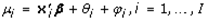 | (2.1) |
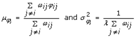 | (2.2) |
 was selected to be conditionally conjugate, that is, conditionally on ϕ the posterior distribution of θj of the same type as
  . Use of a conditionally conjugate prior in our epidemiological, geo-spatiotemporal, hierarchical diffusion-related, district-level, subcounty, COVID-19, stratified, hyper/hypo-endemic, transmission-oriented, vulnerability model allowed deriving and simulating the marginal posterior density π(ϕ∣y). A conjugate prior is an algebraic convenience, giving a closed-form expression for the posterior; otherwise, numerical integration may be necessary (Gelman 2015). Further, according to chapter 3 of Gelman's Data Bayesian Analysis [DBA], when we have yi∼N(μ,σ2)yi∼N(μ,σ2) ,and p(μ,σ2)∝(σ2)−1p(μ,σ2)∝(σ2)−1. Subsequentlyp(μ,σ2|y)∝σ−n−2exp(−12σ2(n−1)s2+n(y¯−μ)2)p(μ,σ2|y)∝σ−n−2exp(−12σ2(n−1)s2+n(y¯−μ)2). We were interested in p(μ|y)=∫p(μ,σ2|y) dσ2p(μ|y)=∫p(μ,σ2|y) dσ2, for which Gelman states the following in page 66 of the third edition of DBA. We assumed that integral may be optimally weighed in the stratified, COVID-19 using the substitution;
 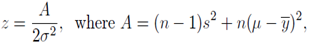 We recognized that the result in the geo-spatiotemporal COVID-19, stratified, aggregation/non-aggregation-oriented, epidemiological, forecast-related, vulnerability-orientedy model used an un-normalized gamma integral hence we deduced:
 Our assumption was conjugate priors may give intuition, by more transparently revealing how a likelihood function updates a prior distribution in an epidemiological, geo-spatiotemporal, hierarchical diffusion-related, district-level, vulnerability, regression model for unbiasedly predictively targeting and prioritizing subcounty, hyper / hypo-endemic, aggregation/non-aggregation-oriented, diagnostically grid-stratifiable, prognosticative, COVID-19, geo-spatiotemporal, geosampled, epidemiological, exogenous estimators. Interestingly, the authors of Jacob et al. (2014) discovered serious problems with the inverse-gamma family of “non-informative” prior distributions. They even considered some proposed non-informative prior distributions in the literature, including uniform and inverse-gamma families, in the context of an expanded conditionally conjugate family. The appropriate specification of priors still contained minimal information. Jacob et. al. (2014) suggests instead to use a uniform prior on the hierarchical standard deviation, employing the half-t family especially when the number of infectious groups is small (e.g., potential “cold spot” geosampled, time series, dependent, subcounty, district-level, viral case data) and in other settings where a weakly informative prior is undesirable. Hence, in this experiment we illustrated the use of the half-t family for geo-spatiotemporal, epidemiological, forecast modelling multiple variance diagnostic, geo-spatiotemporal, hierarchical diffusion-related, COVID-19, diagnostic stratified, epidemiological parameters derived from the hyper/hypo-endemic, aggregation / non-aggregation-oriented determinants such as those that arose in the analysis of variance (ANOVA). We employed a uniform prior on the standard deviation, when the number of diagnostic, hierarchical, diffusion-related, discrete, integer, count values in a Ugandan district was small. A uniform function is simply a function that takes the same value for all its arguments (Gelman 2005). For example, in the geo-spatiotemporal, COVID-19 subcounty, district-level, prognosticative, vulnerability model f(θ)=1,θ∈[0,1] qA was a uniform function. When you take such function as a prior distribution for an unknown parameter θ, you have a uniform prior, also called a flat prior. We also illustrated the usage of time series, predictive, vulnerability-oriented modelling of the variance parameters such as those that arise in the ANOVA.We present a new framework for prior selection based on a hierarchical decomposition of the total variance along a tree structure to the individual geosampled, COVID-19, stratified, epidemiological, forecast-related, subcounty, district-level, aggregation/non-aggregation-oriented, vulnerability model, uncertainty components. The variance parameters in additive models are commonly assigned independent priors that do not account for model structure in an epidemiological, time series, dependent, viral infection, estimation model (Jacob et al. 2014). Hence for each split in the tree, an analyst may be ignorant, or may have a sound intuition on how to attribute variance to the branches. In the former case, a Dirichlet prior may be appropriate to use, while in the latter case a penalized complexity (PC) prior may be assumed to provide robust shrinkage. A bottom-up combination of the conditional priors we further assumed would result in a proper joint prior in our geo-spatiotemporal, epidemiological, forecast-oriented, iterative, interpolation model for optimizing, predictively targeting and prioritizing, aggregation-oriented, COVID-19, district-level, subcounty, hyper-endemic, hot spots. Jacob et al. (2014) suggests default values for the hyperparameters and offers intuitive statements based on expert knowledge for transmission-oriented, hyper/hypo-endemic, prognosticative models. Hyperparameters are parameters whose values control the learning process and determine the values of model parameters (Gelman 2013). The prior framework is applicable for R packages for Bayesian inference such as INLA and RStan.Three simulations showed that, in terms of the application-specific measures of interest, priors improved inference over Dirichlet priors when employed to penalize different levels of complexity in splits in an epidemiological geo-spatiotemporal, forecast-related, vulnerability model for simulating targeting and prioritizing hyper/hypo-endemic, COVID-19 estimators. The parameters were determined using a binomial distribution along with an a priori distribution, and the results had a high degree of accuracy. We assumed that assigning current state-of-the-art default priors for each variance parameter individually may be less transparent in an epidemiological, geo-spatiotemporal, hierarchical, diffusion, forecast-related, vulnerability-oriented, subcounty, COVID-19 stratified model and hence would perform better than using the proposed joint priors. We demonstrate practical use of the new framework by analysing propagation, spatial non-normality (i.e., non-homoscedasticity, non-Gaussianity non-asymptoticalness, geo-spatiotemporal multicollinearity etc.,) heterogeneity in the complex, geosampled, hierarchical, diffusion-oriented, COVID-19,diagnostic, stratified, georeferenced, subcounty, district-level, epidemiological, survey dataset.The Monte Carlo method of error propagation assumed that the distribution of error variables for each of the input data layers generated in PROC MCMC from the regressed, non-homoscedastic, multicollinear, non-asymptotically biased, georeferenced, COVID-19, diagnostically stratified, geosampled, subcounty, district-level determinants were known. To employ PROC MCMC, we needed to specify a likelihood function for the epidemiological data and a prior distribution for the parameters. Since we were fitting hierarchical models, we had to specify a hyperprior distribution and distributions for the RE parameters. In Bayesian statistics, a hyperprior is a prior distribution on a hyperparameter, that is, on a parameter of a prior distribution (Gelman 2013). As with the term hyperparameter, the use of hyper is to distinguish it from a prior distribution of a parameter of the model for the underlying system. Hyperpriors, like conjugate priors, are a computational convenience – they do not change the process of geo-spatiotemporal, generalizable, hierarchical, Bayesian inference, but simply allow one to more easily describe and compute with the prior. ( Lee, Se Yoon; Mallick, Bani 2021).Firstly, we employed a hyperprior which allowed expressing uncertainty in a hyperparameter in the COVID-19, diagnostic, stratified epidemiological, prognosticative model. Quantitating variability in a hyperparameter of the prior allowed conducting a sensitivity analysis and determining a distribution of the hyperparameters which subsequently allowed us to express uncertainty in the geo-spatiotemporal, hierarchical diffusion hyper/hypo-endemic, aggregation/non-aggregation-oriented, propensities in the stratified, clinical, environmental, and socioeconomic, COVID-19, diagnostic determinants. More abstractly, if one employ a hyperprior, then the prior distribution (on the parameter of the underlying model) itself is a mixture density in any epidemiological, geo-spatiotemporal, hierarchical diffusion, aggregation / non-aggregation-oriented, hyper/hypo-endemic, transmission-related, COVID-19, stratified, forecast, vulnerability model for targeting and prioritizing georeferenceable, subcounty, district-level, hot/cold spots: it is the weighted average of the various prior distributions (over different hyperparameters), with the hyperprior being the weighting. This adds additional distributions (beyond the parametric family one is using), because parametric families of distributions are generally not convex sets – as a mixture density is a convex combination of distributions; it will in general lie outside the family. For instance, the mixture of two empirically regressed epidemiological, forecast-related, vulnerability-oriented, subcounty, district-level, COVID-19, diagnostically stratified models’ normal distributions is not a normal distribution: if one takes different means (sufficiently distant) and mix 50% of each, one obtains a bimodal distribution, which is not normal. In fact, the convex hull of normal distributions is dense in all distributions, so in some cases, an infectious disease modeller or researcher can arbitrarily closely approximate a given prior for robustifying geo-spatiotemporal, empirical, hierarchical diffusion-related, vulnerability-oriented, prognosticative, epidemiological, COVID-19, stratifiable, model uncertainty-related, non-normal, estimators for optimally targeting and prioritizing georeferenceable, district-level, subcounty, aggregation-oriented, hyper/hypo-endemic, transmission-related geolocations by using a family with a suitable hyperprior.What makes this approach particularly useful in an aggregation/non-aggregation-oriented, subcounty, district-level, geo-spatiotemporal, hierarchical, diffusion-oriented, COVID-19, stratifiable, hyper/hypo-endemic, diagnostically stratifiable, epidemiological, prognosticative, uncertainty-related model is individual conjugate priors have easily computed posteriors, and thus a mixture of conjugate priors would be the same mixture of posteriors: one only needs to know how each conjugate prior changes in the model to allow for quantitating heteroscedastic, multicollinear or, other biased, variable, uncertainty estimates. Using a single conjugate prior may be too restrictive but using a mixture of conjugate priors may give an infectious disease modeller or other researchers, the desired distribution in a geosampled dataset of regressed diagnostic determinants, a form that is easy to compute with. In this experiment we assumed that the uncertainty non-normal estimator quantification was effective for optimizing diagnostic testing and for eigen-decomposing a function in terms of eigen-spatial filter eigenvectors for determining zero autocorrelated latent estimates and other non-normalities in an epidemiological, stratifiable, COVID-19, prognosticative, aggregation / non-aggregation-oriented, hyper/hypo-endemic, model output.Further, Bayes' theorem calculated the renormalized pointwise product of the prior and the likelihood function, to produce the posterior probability distribution, which in the geosampled, COVID-19, stratified, predictive, vulnerability-oriented model was representable by the conditional distribution of the uncertainty-oriented biased, non-normal quantities derived from the epidemiological, geo-spatiotemporal, subcounty, district-level, regressed, epidemiological data. Similarly, the prior probability or an uncertain proposition in our model was the unconditional probability that was assigned before any relevant evidence was considered. The parameters of the prior distributions were a kind of hyperparameter in the model. Since we employed a beta distribution to model the georeferenced, district-level, time series, dependent, epidemiological, diagnostic, COVID-19 parameters (p) of a Bernoulli distribution, then: p in our model was a parameter of the underlying system (Bernoulli distribution), and α and β were the parameters of the prior distribution (beta distribution); hence hyperparameters. Hyperparameters themselves may have hyperprior distributions expressing beliefs about their values (Gelman et. al. 2013). Since our inferential, subcounty, district-level, georeferenced, vulnerability-oriented, epidemiological, COVID-19, diagnostically stratifiable, prognosticative model had more than one level of prior it was a hierarchical uncertainty-oriented Bayes model. Markovian chains obtained residual, asymptotical, samples from the corresponding posterior distributions, produced summary and diagnostic statistics, and saved the posterior samples in an output dataset which we used for further analysis. Although PROC MCMC supports a suite of standard distributions, we only analysed the district-level, subcounty, COVID-19 stratified, hierarchical, diffusion-oriented estimators employing likelihood priors, and hyperpriors, since these functions were programmable using the SAS DATA step functions. There were no constraints on how the diagnostic, epidemiological parameters would enter the model, in either, linear or any nonlinear, functional form. The MODEL statement in PROC MCMC automatically displayed potential non-homoscedastic, non-asymptotical and multicollinear, aggregation/non-aggregation-oriented, hyper/hypo-endemic, response variable data, in the empirical, estimator, epidemiological, model dataset. In releases before SAS/STAT 12.1, observations with missing values were discarded prior to the analysis. Fortunately PROC MCMC treated the missing values in the COVOD-19 model as unknown parameters and incorporated the sampling of the missing values as part of the simulation. This included quantifying uncertainty about input distribution parameters. PROC MCMC selected a sampling method for each geosampled, hierarchical, diffusion-related COVID-19 stratified, potential, residually skew, non-homoscedastic, non-asymptotical, and or multicollinear, non-normal, parameter estimator from the block of iteratively, interpolated, georeferenced, district-level, diagnostic determinants. Since conjugacy was available, samples were drawn directly from the full conditional distribution by employing standard random number generators. In most cases, PROC MCMC employs an adaptive blocked random walk Metropolis algorithm that employs a normal proposal distribution. In this experiment we were able to choose alternative sampling algorithms [e.g., slice sampler].Metropolis–Hasting methods form a widely used class of MCMC methods for sampling from complex probability distributions (Gelman 2005). It was, therefore, of considerable interest for us to develop mathematical analyses which explained the structure inherent in these algorithms, especially for articulating erroneous structure in our prognosticative, epidemiological, Bayesian, subcounty, district-level, stratifiable, COVID-19, vulnerability-related, geo-spatiotemporal, parameter, estimation model which we assumed would be pertinent to understanding the computational complexity of the uncertainty algorithm. We further assumed that quantifying computational complexity of an MCMC method would be most naturally undertaken by studying the behavior of the method on a family of probability distributions indexed by our autoregressive, semi-parameterizable, COVID-19, diagnostically stratifiable, georeferenced, geo-spatiotemporally dependent, hierarchical, diffusion-oriented, vulnerability-related prognosticative, epidemiological estimators. Doing so we assumed would allow studying the cost of the algorithm in terms of uncertainty generation while quantitating the propagation non-normality (i.e., biased, non-homoscedasticity geo-spatiotemporal multicollinearity, zero autovariance), in the aggregation/non-aggregation-oriented, hyper / hypo-endemic, asymptotical, estimator, empirical dataset. In this experiment we studied the cost as a function of dimension for algorithms applied to a family of probability distributions derived from finite dimensional approximation of a measure on an infinite-dimensional space for optimally quantitating hyper/hypo-endemic, heteroscedastic, multi-collinear, and other non-normal, COVID-19, stratified, hierarchical diffusion-transmission-oriented subcounty, district-level, determinants.We also proposed a more efficient version of the slice sampler for Dirichlet process mixture models. The Dirichlet process is a stochastic process employed in Bayesian nonparametric models of data, particularly in Dirichlet process mixture models (also known as infinite mixture models). It is a distribution over distributions, i.e., each draw from a Dirichlet process is itself a distribution. (Cressie 1993) We assumed this sampler would allow the fitting of infinite mixture, vulnerability-related, epidemiological, district-level, COVID-19, diagnostically stratified, geo-spatiotemporal, regressively forecastable, hierarchical, diffusion-oriented, model estimators with a wide–range of prior specification for optimally prioritizing and targeting hyper/hypo-endemic, georefernceable, subcounty, hot/cold spot, transmission-related, aggregation/non-aggregation, hyper/hypo-endemic sites. We then stepped through the various constructions of the Dirichlet process, outlined a number of the basic properties of this process and moved on to the mixture of Dirichlet processes model. To illustrate this flexibility, we developed a nonparametric prior for the mixture model by normalizing a sequence of independent, hierarchical, diffusion-oriented, COVID-19, diagnostic variables and showed how the slice sampler can be applied to make inference in a normalized, subcounty, district-level, transmission-related, vulnerability model constructed in R.The bayes4psyR package provided a state-of-the art framework for our, geo-spatiotemporal, hierarchical diffusion, uncertainty-oriented, Bayesian autocorrelation, analysis using the subcounty, district-level, empirical, georeferenced, epidemiological, diagnostic data. The analyses incorporated a set of probabilistic, forecast-oriented, vulnerability-related, uncertainty, estimation models for inspecting the non-homoscedastic, multicollinear parameters and other non-normal epidemiological data. All models were pre-compiled, meaning that we did not need any specialized software or skills (e.g., knowledge of probabilistic programming languages). The only requirements for building our time series, estimation, Bayesian model was inputting the empirical georeferenced dataset of aggregation/non-aggregation-oriented, COVID-19, stratified, diagnostic determinants into R programming language. R is one of the most powerful and widespread programming languages for statistics and visualization. The package incorporated the diagnostic, analytic and visualization tools required for conducting the time series, Bayesian data analysis in eigenvector eigen-geospace. For statistical computation (sampling from the, georeferenced, COVID-19 stratified, district-level, predicted, posterior distributions) in the bayes4psy package, we utilized Stan. Stan is a state-of-the-art platform for statistical modelling and high-performance statistical computation which offers full Bayesian statistical inference with MCMC sampling. Visualizations in the bayes4psy package for constructing our epidemiological, geo-spatiotemporal, hierarchical, diffusion-oriented, hyper/hypo-endemic, prognosticative, georeferenced, empirical, aggregation/non-aggregation-oriented, district-level, subcounty, COVID-19 model was based on the ggplot2 package.Two sub-models were studied in detail. The first one assumed that the positive random variables generated from the regressed, time series, dependent, aggregation/non-aggregation-oriented, COVID-19, stratified, hierarchical, diffusion-related, epidemiological data, georeferenced, capture points were Gamma distributed and the second assumed that they were inverse–Gaussian distributed. Both priors had two hyperparameters and we considered their effect on the prior distribution based on the total number of non-normal, grid-stratifiable COVID-19, specified, “hot/cold spot”, district-level, subcounty, diagnostic determinants. Extensive computational comparisons with alternative “conditional” simulation techniques for mixture models were applied using the standard Dirichlet process prior and a new prior was generated. The properties of the new prior generated from the model were illustrated for implementing a density error estimation procedure. We show that the discreteness of the Dirichlet process can have a large effect on inference (posterior distributions and Bayes factors) in an epidemiological geo-spatiotemporal, hierarchical, diffusion-oriented, COVID-19, diagnostically stratified, sub-county, district-level epidemiological, forecast model, for prioritizing and targeting district-level, subcounty, hyper/hypo-endemicity leading to conclusions that can be different from those that result from a reasonable semi-parametric model. When the observed data are all distinct, the effect of the prior on the posterior is to favor more evenly balanced partitions, and its effect on Bayes factors is to favour more groups (Gelman et.al,2013). Henceforth, when constructing an epidemiological, hierarchical, diffusion-oriented, diagnostic, COVID-19, stratified, forecast-related, vulnerability model with a Dirichlet process as the second-stage prior, the prior can have a large effect on inference, but in the opposite direction, towards more unbalanced partitions.Subsequently, each of the data layers and an error surface was simulated by drawing, at random, from an error pool as defined by the geographic distribution of the district-level, georeferenced, COVID-19, epidemiological, grid-stratified, diagnostic variables. Error surfaces were added to the input data layers and to the parameter estimators. A model was run using the resulting data error layers as input. The process was repeated so that, for each run, a new realization of an error surface was generated for each input data layer. The results of each run were accumulated and a running mean and standard deviation surface for the output was calculated. This process continued until the running mean stabilized. Since the random error visualizations were both positive and negative, the stable running mean were taken as the true model output surface, and the standard deviation surface was employable as a residual measure of relative non-normality in the aggregation/non-aggregation-oriented, prognosticative, variable, estimation error. A simple summary was generated, showing posterior mean, median and standard deviation, with a 95% posterior credible interval.Models were compared employing the Deviance Information Criterion (DIC) in PROC MCMC where
 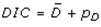 , was the sum of the posterior mean of the deviance, (D), a measure of goodness-of-fit, and the effective number of diagnostic, georeferenced geosampled, district-level, subcounty, epidemiological, time series, dependent, normalized, hierarchical diffusion, hyper / hypo-endemic, aggregation/non-aggregation-oriented, COVID-19 stratified, diagnostic parameters (pD). A measure of goodness-of-fit based on the DIC values was applied and an R2DIC was calculated in line with the standard R2 measure for the geo-spatiotemporal, iterated, residual forecasts (i.e., subcounty, temporally targeted, district-level, hyper/hypo-endemic, aggregation / non-aggregation-oriented hot/cold spots). These were optimally definable employing:
  when DICk was the DIC value for sub-model k under evaluation and when DICmax was the DIC value for one-fixed parameter model; and,
  was the posterior deviance as derived iteratively from the model.Model checking of all data input and compilation was conducted in PROC MCMC. The number of chains had to be specified before compilation. For constructing our vulnerability-oriented, prognosticative, epidemiological, time series, hierarchical, diffusion-related, district-level, georeferenceable, Bayesian, uncertainty model, three parallel chains were run. Syntax checking was employed, which involved highlighting the entire model code and then choosing the sequence model specification. The uncertainty-related non-normal quantities in the estimates derived from the MCMC sequence of the random, epidemiological, time series, dependent, COVID-19, stratified, diagnostic samples were subsequently determined by Nk and vk. These estimates also revealed a PDF [i.e., a statistical expression that defined a probability distribution and the likelihood] of the district-level, aggregation / non-aggregation-oriented, transmission-related, subcounty site being a hyper/hypo-endemic, COVID 19, hot/cold spot based on a regression outcome. Here every individual, discreetly, exogenously geosampled, hierarchical, diffusion-related, explanatory variable [e.g., a grid-stratifiable, georeferenced, endemic, transmission-oriented, clinical, environmental, or socioeconomic diagnostic determinant was invasively examined (as opposed to quantitating a continuous random variable) using a scalar quantity v. The estimated value of v in the vulnerability-oriented, COVID-19, subcounty, district-level model was provided by the sample mean,
  We then addressed the problem of upper bounding the MSE of the MCMC estimators. Our analysis was asymptotic. We first established a general result valid for all ergodic Markov chains encountered in the Bayesian computation and at multiple unbounded target functions. The bound was sharp in the sense that the leading term was exactly σ2(P,f)/nσas2(P,f)/n, where σ2 was(P,f)σ2(P,f) which was the CLT asymptotic variance. In probability theory, the CLT establishes that, in situations when independent random variables are summed up, their properly normalized sum tends toward a normal distribution even if the original variables themselves are not normally distribute.Next, we proceeded to specify additional assumptions and generated explicit computable bounds for geometrically and polynomial ergodic Markov chains under quantitative drift conditions. We generated quantitative bounds on the convergence rates of Markov chains, under conditions implying polynomial convergence rates. This paper extends an earlier work by Roberts and Tweedie (Stochastic Process. Appl. 80(2) (1999) 211), which provides quantitative bounds for the total variation norm under conditions implying geometric ergodicity. Explicit bounds for the total variation norm were obtained for the subcounty, district-level, COVID-19, stratified, epidemiological, prognosticative, vulnerability model by evaluating the moments of an appropriately defined coupling time, employing a set of drift conditions, adapted from an earlier work by Tuominen and Tweedie (Adv. Appl. Probab. 26(3) (1994) 775). Applications of the model result were then presented to study the convergence of random walk Hastings Metropolis algorithm for generating super-exponential target functions and general state-space models. Like the MCMC, the Metropolis-Hastings algorithm is used to generate serially correlated draws from a sequence of probability distributions. The sequence converges to a given target distribution. Explicit bounds for f-ergodicity were given for the COVID-19 model for an appropriately defined control function f. As a corollary, we provided results on confidence estimation.The expected variance
  was the expectation for the ensemble of the sequences as robustly parsimoniously rendered from the georeferenced, aggregation / non-aggregation-oriented, hyper/hypo-endemic, regressed, geo-spatiotemporal, epidemiological, geosampled, hierarchical, diffusion-related, endemic, diagnostic, MCMC estimators which in this experiment we expressed as:
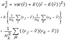 where
where 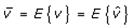 . The autocovariance of the sequence was definable as:
 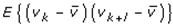 . The asymptotical normalized, non-zero autocovariance was
 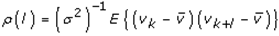 , where σ2 was the variance of v and ρ (l) did not depend on k. The length of the non-zero, derived, normalized, autocovariance geo-spatiotemporal values was then optimally determined by
 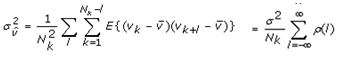 . Here the normalized autocovariance was a symmetric function, i.e., ρ (-l) = ρ (l). The sequence sufficiently converged to the target PDF. The variance of the distribution of the, non-skew, homoscedastic, non-multi-collinear, asymptotically normalized, aggregation / non-aggregation-oriented, hierarchical, diffusion-related, COVID-19, stratified, diagnostic estimators was generated employing
 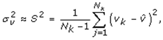 The normalized autocovariance was derivable from the sequence employing:
  for lag l ≥ 0.Henceforth, an MCMC sequence derived from an empirical geosampled dataset of georeferenced, skewed, non-homoscedastic, and or multicollinear, multivariate, non-asymptotical, aggregation/non-aggregation-oriented, geo-spatiotemporal, COVID-19, biased, hierarchical, diffusion-related, geo-spatiotemporal, non-normal paradigm is definable as the reciprocal of the ratio of the number of MCMC trials needed to achieve homogenous variance in any estimated uncertainty quantity. In this experiment the MCMC sampled were synthesizable from independent draws from the target PDF as quantitatively iterated from the georeferenced, uncertainty-oriented, COVID-19 model, specified, diagnostic prognosticators. The estimation of the mean and the variance for independent, time series, dependent, empirical estimators were calculable by:
  . After compilation, the files contained a portion of the initial geosampled values for the parameters selected in the model. After careful inspection of the data, no aberrant values, leading to numerical overflow were found.The aggregation/non-aggregation-oriented, normalized, residual estimates as extracted from the diagnostic, hierarchical, diffusion-related, COVID-19, stratified, district-level, georeferenced, asymptotical, vulnerability-related, epidemiological, sub-county, hyper/hypo-endemic model forecasts were subsequently evaluated in a spatial error model. An autoregressive model was incorporated that employed the geo-spatiotemporal, indexable, hierarchical diffusion-oriented, homoscedastic, non-multi-collinear, exogenous predictors, Y, as a function of nearby diagnostic, clinical, socioeconomic or environmental, grid-stratifiable, georeferenceable, COVID-19, stratifiable, parameter estimator geosampled, Y values [i.e., an autoregressive response (AR), or spatial linear (SL) specification], and/or the residuals of Y as a function of nearby district-level Y residuals [i.e., an AR or SE specification]. Distance between the georeferenced, sub-county, epidemiological, capture points was subsequently definable in terms of an n-by-n geographic weights matrix, C, whose cij values were 1 if the specified, time series dependent, district-level geolocations i and j were deemed nearby, and 0 otherwise. Adjusting this matrix by dividing each row entry by its row sum, with the row sums given by C1, converted this matrix-to-matrix W. The n-by-1 vector x = [x1 ⋯ xn] T contained measurements of quantitative, potential, hierarchical, diffusion-related, homoscedastic, non-multicollinear, asymptotical diagnostic determinants for n spatial units and n-by-n weighting matrix W. The formulation for the Moran's I of spatial autocorrelation for the time series, epidemiological, diagnostic model was subsequently computed employing
  where
where  with i ≠ j. The values wij were spatial weights stored in the symmetrical matrix W [i.e., (wij = wji)] that had a null diagonal (wii = 0). Here, the matrix was initially fit to an asymmetrical matrix W. Matrix W was generalizable by a non-symmetric matrix W* by rigorously employing W = (W* + W*T)/2. Subsequently, the Moran's I was rewritten employing the matrix notation:
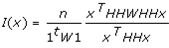
 where H = (I - 11T/n) was an orthogonal projector verifying that H = H2, (i.e., H was independent).A spatially autoregressive (SAR) model specification was subsequently employed to describe the autoregressive variance, geo-spatiotemporal, non-zero autocorrelatable, non-multicollinear, asymptotical, unbiased, forecasted, aggregation/non-aggregation-oriented estimates. A spatial filter model specification was employed to describe both heterogeneous, Gaussian and Poisson, random, diagnostic, COVID-19 stratified, hyper/hypo-endemic hierarchical, diffusion-related, diagnostic, determinant effects. The resulting SAR model specification took on the following form:
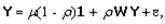 | (2.1a) |
 | (2.2a) |
 parsimoniously enabled positing a positive relationship between the grid-stratified, time series, dependent, georeferenced, COVID-19, diagnostically stratifiable, hierarchical, diffusion-related, non-zero, autocorrelated covariates when y1 and y2, had a negative relationship between covariates, y3 and y4, and no relationship between covariates y1 and y3 and between y2 and y4. This covariance specification yielded:
 | (2.3a) |
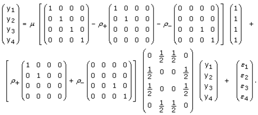 If either ρ+ = 0 (and hence I+ = 0 and I- = I) or ρ- = 0 (and hence I- = 0 and I+ = I), then equation (2.3) reduced to equation (2.1). This indicator variable classification was made in accordance with the quadrants of the corresponding Moran scatterplot created using the georeferenced, district-level, COVID 19, stratified hierarchical, diffusion-related, geo-spatiotemporal, transmission-oriented, hyper/hypo-endemic, subcounty, aggregation / non-aggregation-oriented, empirical, diagnostic determinants in PROC AUTOREG.If PSA and NSA processes counterbalance each other in a mixture, the sum of the two spatial autocorrelation parameters--(ρ+ + ρ.) will be close to 0 (Griffith 2003). Here, Jacobian estimation was implementable by utilizing the non-homogenous, diagnostic, indicator values derived from the eigendecomposed, eigen-orthogonal, eigen-spatial filter geosampled, aggregation/non-aggregation-oriented, district-level, hyper/hypo-endemic, temporally stratified, COVID-19, hierarchical diffusion-related, exogenous variables (I+ - γ I-) in eigenvector eigen-geospace which required estimating ρ+ and γ with ML techniques, and setting
  Most of the literature to date proposes approximations to the determinant of a positive definite n × n spatial covariance matrix (i.e., the Jacobian term) for Gaussian spatial autoregressive models that fail to support the analysis of non-normal estimator quantification in massive, georeferenced, geo-spatiotemporal, epidemiological, variable, estimator datasets. We employed a much simpler Jacobian approximation whereby selected eigenvalue estimation techniques summarized validation results for approximating the eigne-orthogonal eigen-spatial, filter, non-zero, synthetic, eigenvalues in eigenvector eigen-geospace. Jacobian approximations, and an estimation of a spatial autocorrelation parameter was usable to illustrate the spatial autocorrelation, stratified, parameter in the autoregressive, aggregation/non-aggregation-oriented, hyper/hypo-endemic, hierarchical, diffusion-related, epidemiological, district-level, prognosticative, COVID-19, model specification. One of the principal contributions of this paper was the implementation of an autoregressive model specification for any size empirical dataset of non-skew, homoscedastic, non-multicollinear, non—biased. non-zero autocorrelatable, geo-spatiotemporally forecastable, asymptotically normalized, uncertainty–free, geo-spatiotemporal, vulnerability-oriented, hyper/hypo-endemic, transmission-related, COVID-19, diagnostic determinants. Its specific additions to the literature henceforth include (1) new, more efficient estimation algorithms; (2) an approximation of the Jacobian term for epidemiological geosampled data forming complete rectangular regions [i.e., hyper-endemic, georeferenceable, subcounty, district-level, hot spots; (3) issues of inference; and (4) timing results.The Jacobian generalized the gradient of a scalar-valued function of multiple, georeferenced, district-level, hierarchical, diffusion-related, COVID-19 stratified sub-county, aggregation/non-aggregation-oriented, non-skewed, non-zero autocorrelated, predictor variables which itself generalized the derivative of a scalar-valued function of a scalar. A more complex specification was subsequently posited by generalizing these binary indicator, time series, dependent, explanatory variables in eigenvector eigen-geospace. We employed F: Rn → Rm as a function from Euclidean n-space to Euclidean m-space, which was derivable employing the Euclidean, distance between the hierarchical, diffusion-related, epidemiologically specifiable, clinical, environmental and socioeconomic, diagnostic determinants and a hyper/hypo-endemic, forecasted, district-level, subcounty, hot/cold spot estimator. Such a function was given by m covariate (i.e., component functions), y1(x1, xn), ym(x1, xn). The partial derivatives of all these functions were organized in an m-by-n matrix; the Jacobian matrix J of F, which was parsimoniously displayable as follows:
 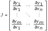 This matrix was denotable by JF (x1, xn) and
  . The ith row (i = 1, m) of this matrix was the gradient of the ith component function yi: (∇ yi). In this experiment, p was an empirical epidemiological, geo-spatiotemporally, dependent, hierarchical, diffusion-related, eigendecomposed, eigenfunction, eigen-spatial filtered, non-skew, homoscedastic, non-multicollinear, asymptotically unbiased, non-zero autocorrelatable, determinant in Rn, but only when F (i.e., geosampled, district-level, COVID-19, diagnostically stratified, subcounty case count) was differentiable at p; its derivative was hence subsequently extractable by JF(p). The model described by JF(p)) was the best linear approximation of F near a georeferenced, sub-county, district-level, geo-spatiotemporal, COVID-19 stratifiable, epidemiological, sentinel site, capture point p, in the sense that:
 | (2.4) |
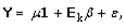 | (2.5) |
 and
and  for equation (2.3). Expressing equation (2.3) in terms of the preceding 2-by-2 example yielded
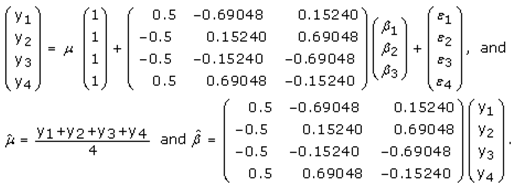 Of note is that the 2-by-2 square tessellation rendered a repeated eigenvalue in the COVID-19, vulnerability-oriented, epidemiological, residual, prognosticative, model output.To identify subcounty, georeferenceable, district-level, clusters of, asymptotically normalized, non-zero autocorrelatable, geo-spatiotemporal, hierarchical, diffusion-related, diagnostically stratified, COVID-19, homoscedastic, non-multicollinear, hyper/hypo-endemic, determinants, Thiessen polygon surface partitionings were generated in ArcGIS ProTM for constructing neighbour matrices, which also were employable in the probabilistic, latent, autocorrelation eigenvector, eigen-spatial, filter, eigen-analysis. Entries in matrix were 1, if two georeferenced, explanative, grid-stratifiable, COVID-19, geosampled, diagnostic covariates shared a common Thiessen polygon boundary and 0, otherwise. Next, the linkage structure for each surface was edited to remove unlikely geographic neighbours to identify pairs of dependent, explanatory, hierarchical, diffusion-related, georeferenced, diagnostic, aggregation/ non-aggregation-oriented determinants sharing a common district-level Thiessen polygon boundary. Attention was restricted to those map patterns associated with at least a minimum level of spatial autocorrelation, which, for implementation purposes, here, was optimally definable by |MCj/MCmax| > 0.25, when MCj denoted the jth value and MCmax, the maximum value of MC. This threshold value allowed two candidate sets of eigenvectors generated by the eigenfunction eigen-decomposition of the district-level, subcounty, time series, hierarchical, diffusion-oriented, geosampled, diagnostic estimators to be considered for substantial PSA and NSA respectively. These statistics indicated that the detected NSA in the time series, dependent, epidemiological, COVID-19, diagnostically stratified, hierarchical, diffusion-related, estimator dataset could be statistically non-significant, based upon a randomization perspective. Of note, is that the ratio of the PRESS (i.e., predicted error sum of squares) statistic to the sum of squared errors from the MC scatterplot trend line was 1.21 which was well within two standard deviations of the average standard prediction error value (roughly 1.11) for a georeferenced, diagnostic, COVID-19, stratified, subcounty, district-level, geosampled, hierarchical, diffusion-oriented, asymptotically unbiased, non-skew, homoscedastic, geo-spatiotemporal, normalized, non-multicollinear, non-zero, autocorrelatable, aggregation/non-aggregation-oriented, hyper/hypo-endemic, transmission-related, asymptotical, explanatory variable.Because counts were being analysed, a Poisson spatial filter model specification was employed to fit the district-level, COVID-19, estimators. Detected overdispersion (i.e., extra-Poisson variation) results in its mean being specified as gamma distributed (Haight 1967). The model specification was written subsequently as:
  where μi was the expected mean, derived from the COVID-19, specified case count, district-level, geolocation i, μ was an n-by-1 vector of expected case counts, LN denoted the natural logarithm (i.e., the GLM link function), α was an intercept term, and η was the negative binomial dispersion parameter. This log-linear equation had no error term; rather, estimation was executed assuming a negative binomial random variable.The upper and lower bounds for a spatial matrix generated employing Moran’s I was subsequently deduced by λmax (n/1TW1) and λmin (n/1TW1) where λmax and λmin which in this experiment were the extreme eigenvalues of Ω = HWH in the geosampled, COVID-19, stratified, epidemiological model, eigen-decomposed eigen-spatial, filter, synthetic, eigen-orthogonal eigenvectors. The eigenvectors of Ω were vectors with unit norm maximizing Moran's I. The eigenvalues of this matrix were asymptotically synthesizable from the geo-spatiotemporal, semi-parameterized, diagnostic, empirical geosampled dataset which was equal in value to the Moran's I coefficients derived from the residual autocorrelation post-multiplied by a constant. Eigenvectors associated with high positive (or negative) eigenvalues have high positive (or negative) autocorrelation (Griffith 2003). The synthetic, eigen-function, eigen-decomposed, eigen-orthogonal, eigenvectors associated with extremely small hierarchical, diffusion-related, discrete, integer values corresponded to 0 autocorrelation, subcounty geolocations, (i.e., z scores =0) and were not suitable for defining spatial structures corresponding to district-level, aggregation / non-aggregation-oriented sites (i.e., subcounty, hot/cold spots of hyper/hypo-endemic, COVID-19 infection rates).The diagonalization of the geospatial uncertainty-oriented, weighting matrix generated for non-heuristically quantitating the autocovariance of the georeferenced, time series, dependent, potential, spatially biased, non-homoscedastic, multicollinear, hyper/hypo-endemic, hot/cold spot aggregation/non-aggregation-oriented, transmission-related geosampled, hierarchical, diffusion-related, COVID-19 stratified, asymptotical, diagnostic determinants consisted of finding the normalized vectors ui stored as columns in the matrix U = [u1 ⋯ un], This satisfied Λ = diag (λ1 ⋯ λ n),
  and
and  for i ≠ j. Note that double centering of Ω implied that the geo-spatiotemporal, eigen-spatial filter, eigen--orthogonal eigenvectors rendered from the eigen-decomposed, COVID-19 stratified, subcounty, district-level, exogenous, regressors were centered and at least one eigenvalue was equal to zero. Introducing these eigenvectors in the original formulation of Moran's I led to:
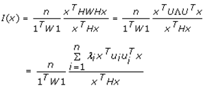 | (2.6) |
 | (2.7) |
 | (2.8) |
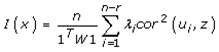 | (2.9) |
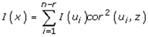 in PROC AUTOREG. The term cor2 (ui, z) represented the part of the variance of z that was explainable by ui in the COVID-19, forecast model when z = β i ui+ ei. This quantity was equal to
  . By definition, the eigenvectors ui were eigne-orthogonal, and therefore, regression coefficients of the linear models z = β i ui+ ei were those derivable from the regression model z = Uβ + ε = β iui + ⋯ + β n-r un-r + ε.The maximum value of 1 was quantifiable by all of the variation of z, as parsimoniously expounded by the eigenvector u1, which corresponded to the highest eigenvalue λ1 in the weighted, autocorrelation, uncertainty matrix constructed from the georeferenced, time series. Here, cor2 (ui, z) = 1 (and cor2 (ui, z) = 0 for i ≠ 1) and the maximum value of I, was intuitively deducible for Equation (2.9), which was equal to Imax = λ1(n/1TW1). The minimum value of I in the error matrix was obtainable as with all the variation of z which in this experiment was definable by the eigenvector un-r corresponding to the lowest eigenvalue λn-r extractable in the forecast model renderings. This minimum value was equal to Imin = λn-r (n/1TW1). If the geosampled, district-level, georeferenced, hierarchical, diffusion-related, explanatory, predictor variable was not definable due to presence of heteroscedasticity multicollinearity, or non-asymptoticalness, the part of the variance explained by each eigenvector was equal, on average, to cor2 (ui, z) = 1/n-1. Because the forecasted explanatory, COVID-19, diagnostic, subcounty, district-level, georeferenceable, epidemiological variables in z were randomly permuted, it was assumed that we would obtain this result.
3. Results
- We considered a Poisson model for count data, y∼Poisson(θ), θ≥0. The parameter θ was interpreted as the prevalence of district-level, COVID-19, and importantly, E[y]=Var(y)=θ. An unfortunate property of the Poisson model is that it cannot model overdispersed data or data in which the variance is greater than the mean (Haight 1967). This is because Poisson regression has one free parameter. However, we placed a gamma prior on θ, yθ ∼Poisson(θ)∼gamma(r,1−pp), and then marginalized out θ, in PROC REG which rendered a negative binomial (NB) distribution, which has the useful property that its variance can be greater than its mean. The derivation for the sub-county, district-level epidemiological regression model was calculable as:
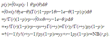 This held in the hierarchical diffusion, epidemiological, COVID-19, count, variable model because of the following equality, ∫0∞xbe−axdx=ab+1Γ(b+1). The Gamma Poisson Distribution PDF for the epidemiological model was
 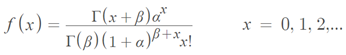 We acclaim that this is part of the usefulness of the gamma function: integrals of expressions of the form f(x)e−g(x), can model exponential decay, in an epidemiological, prognosticative, risk-related, diagnostically stratifiable, COVID-19, explanatory, count variable, regression equation for optimally targeting sub-county, district-level, diagnostic covariates of hierarchical diffusion of the virus which in this experiment was solved using Γ(x)=(x−1)!.in a closed form.The grid-stratified, COVID-19, subcounty, district-level, epidemiological, count data had incidence of zeros greater than expected for the underlying probability distribution which we modelled with a zero-inflated distribution. The district population was considered to consist of two sub-populations. Hierarchical diffusion–related, subcounty, district-level, epidemiological observations drawn from the first subpopulation were realizations of a random variable that typically in this experiment had either a Poisson or negative binomial distribution, which contained zeros. Observations drawn from the second sub-population provided a zero count. Suppose the mean of the underlying Poisson or negative binomial distribution is
  and the probability of an observation being drawn from the constant distribution that always generates zeros is
  ; the parameter
  then will have zero-inflation probability (Haight 1967).The probability distribution of a zero-inflated, Poissonian, random variable Y in our epidemiological, COVID 19, vulnerability-related, prognosticative model was given by
 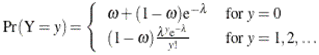 The mean and variance of Y for the zero-inflated Poissonian was given by
 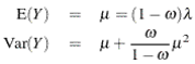 The parameters
  and
and  was subsequently modelled as functions of linear predictors,
 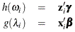 where
where  was one of the binary link functions: logit, probit, or complementary log-log. The log link function is typically used for
  (Freedman 2008). In our subcounty, district-level, COVID-19 epidemiological, forecast model, the underlying Poissonian distribution for the first subpopulation was assumed to have a variance that was equal to the distribution’s mean. However, this was an invalid assumption, as the data exhibited overdispersion.A useful diagnostic tool that can aid in detecting overdispersion is the Pearson chi-square statistic (Freedman 2008). In this experiment Pearson’s chi-square statistic was defined as
  in PROC FREQ. Pearson's chi-squared test was used to assess three types of comparison: goodness of fit, homogeneity, and independence in the COVID19 estimators. A test of goodness of fit established whether an observed frequency distribution in the sub-county, district-level, COVID-19, stratified epidemiological, forecast, vulnerability model differed from a theoretical distribution. This statistic had a limiting chi-square distribution, with df equal to the number of stratified, hierarchical, diffusion-oriented, geosampled observations minus the number of diagnostic parameters estimated. Comparing the computed Pearson chi-square statistic to an appropriate quantile of a chi-square distribution with
  df constituted in this experiment as a test for overdispersion.If overdispersion is detected, the ZINB model often provides an adequate alternative (Haight 1967). The probability distribution of our subcounty, district-level, epidemiological, zero-inflated, negative binomial, random variable Y in the COVID-19 model was given by
  where
where  was the negative binomial dispersion parameter.The mean and variance of Y for the zero-inflated negative binomial was subsequently given by
 and
and  Because our ZINB model assumed a negative binomial distribution for the first component of the mixture, it had a more flexible variance function. Thus, it provided a means to account for overdispersion which was not due to the excess zeros geosampled in the empirical dataset. However, the negative binomial, and thus the ZINB model, achieved this additional flexibility at the cost of an additional parameter. Henceforth, if an epidemiologist, viral infectious disease modeller, or research collaborator fits a subcounty, district-level, potentially residually non-homoscedastic, multi-collinear, prognosticative, vulnerability-oriented, COVID-19, epidemiological, ZINB model and there is no overdispersion, the diagnostic non-asymptotical parameter estimators may be deemed less efficient compared to the more parsimonious ZIP model. The district-level, epidemiological, COVID-19, stratified, hierarchical diffusion, specified, explanatory, parameterized estimator, zero-inflated, Poisson probability model fitting exercise first estimated an RE term together with an intercept and a coefficient for the time covariate number-of-days, given by equation (2.3), and then decomposed this RE term into a SSRE and a SURE component. Consequently, we were able to portray the scatterplot of predicted versus observed values for the combination of contagion and the hierarchical, diffusion-related, parameter estimator, residual effects. Once the independent variables that you wish to retain in the model are identified, and there is a theoretical basis for thinking that the relationships may differ by space, GWR may be an appropriate next step (Griffith 2003). We attempted to exam the empirical, georeferenced dataset of epidemiological time series, dependent, non-homoscedastic, multicollinear, aggregation-oriented, geo-spatiotemporal, variables (e.g., “Median household income’) at the census tract subcounty, georeferenceable, district level using various GWR related paradigms. OLS models were initially run to determine the global regression coefficients (β) for the independent variables: yi = β0 + β1x1i + β2x2i +…+ βnxni + Ɛi with the estimator: β’ = (XT X)-1 XT Y The regression models that underlie our GWR were formulated as yi = β0 + β1x1i + β2x2i +…+ βnxni + Ɛi with the estimator: β’(i) = (XTW(i) X)-1XTW(i)Y where W(i) was a matrix of weights specific to the epidemiological, geo-spatiotemporal, hierarchical, diffusion-related, COVID-19, forecast-oriented, vulnerability model. The prognosticated regression residuals revealed the raw, geosampled, hierarchical, diffusion-related, epidemiological subcounty district data was non-normal. The following models were then studied: (i) GWR with a fixed distance or (ii) an adaptive distance bandwidth (GWRa), (iii) flexible bandwidth GWR (FB-GWR) with fixed distance: and (iv) adaptive distance bandwidths (FB-GWRa), (v) eigenvector spatial filtering (ESF), and (vi) RE-ESF (RE-ESF). Results revealed that the epidemiological, district-level, prognosticative COVID-19 models designed to capture scale dependencies in local relationships (FB-GWR, FB-GWRa and RE-ESF) most accurately estimated the simulated VCMs where RE-ESF was the most computationally efficient. Conversely GWR and ESF, where SVC estimates are naively assumed to operate at the same spatial scale for each relationship, performed poorly. Results also confirm that the adaptive bandwidth GWR models (GWRa and FB-GWRa) were superior to their fixed bandwidth counterparts (GWR and FB-GWR) for predictively targeting and prioritizing, hierarchical diffusion-related, district-level, sub-county, aggregation-oriented, potential, hyper/hypo-endemic, transmission-related, georeferenceable, stratified, COVID-19 hot/cold spots.The scatterplot revealed classical V-shaped dispersion capture points [i.e., georeferenced, subcounty, diagnostic, hyperendemic, aggregation sites] with increasing infectious rates that was characterized by a Poissonian random variable. Because the mean and variance were the same in the vulnerability-oriented, COVID-19, district-level, forecast model, the deviations from the trend line tended to increase with increasing rates. Matrix (I – 11T/27) Cs(I – 11T/27) had five, whereas matrix (I – 11T/31)CH(I – 11T/31) had eight, eigenvectors with PSA satisfying the condition MCj/MC1 > 0.25. Table 1 summarizes results for these two cases, revealing that a hierarchical structure potentially non-homoscedastic, multicollinear, non-asymptotical, eigen-orthogonal eigenvector was very prominent, and that its contagion spatial structure component exhibited strong PSA in the hierarchical diffusion-related, time series, dependent, geosampled, district-level, subcounty, gridded, COVID-19, diagnostically stratifiable, georeferenceable, vulnerability-oriented, epidemiological, prognosticative, model output Eigen-autocorrelation played a prominent role in the derivation of the RE term. Positive geo-spatiotemporal autocorrelation (PSA0 means that geographically nearby values of a variable tend to be similar on a map: values tend to be located near values, (e.g., socio-economic values near other similar attribute feature values). (Griffith 2003)
|
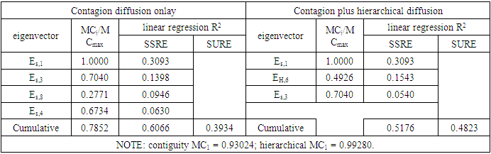
|
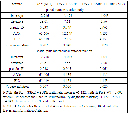
|
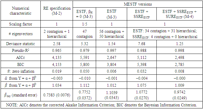
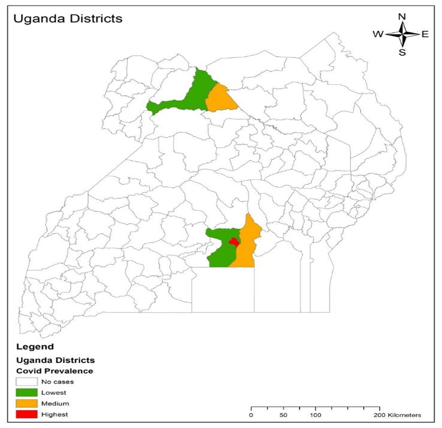 | Figure 1. The MESTF map of COVID-19 transmission due to, hierarchical diffusion diagnostic covariates at the district level in Uganda |
 –[22.18609/(1+e^6.97888 )]^2 + [-0.00037day^2+22.18609 /(1+e^(6.97888-0.18220×day) )]^2.
4. Discussion
- This paper initially investigates multicollinearity, skew-heteroscedasticity and other non-normalities embedded in local Poissionian and GWR coefficients at a single, district-level, subcounty, grid-stratified geolocation, employing an empirical geosampled dataset for precisely identifying geo-spatiotemporal, hierarchical, diffusion-oriented, COVID-19, stratified, epidemiological, diagnostic, hyper/hypo-endemic determinants In this experiment, GWR constructed a separate OLS equation for every potential, geo-spatiotemporal, hierarchical, diffusion, district-level, geolocation in the Ugandan, empirical estimator dataset, which incorporated the dependent, explanatory, diagnostic, determinants falling within the bandwidth of each target, georeferenced, subcounty, geospatial cluster (i.e., potential hyper-endemic hot spot), transmission-oriented geolocation. Bandwidth can be manually entered by the user (based on previous literature (e.g., Griffith 2003)), or it can be determined by the statistical software. Here, a first set of OLS models were initially run in R, to determine the bandwidth. If the bandwidth is not manually entered by an investigator, or epidemiologist most software problems allow the investigator to select the default or “adaptive” bandwidth, which is recommended in the literature (e.g., Chen 2014).Here OLS, hierarchical, diffusion-oriented models were run to determine the global regression coefficients (β) for the independent variables: yi = β0 + β1x1i + β2x2i +…+ βnxni + Ɛi with the estimator: β’ = (XT X)-1 XT Y [Eqn1.5]. Once the epidemiologically, diagnostic, time series, dependent, COVID-19, stratified, independent variables were retained in the district-level, subcounty, forecast-oriented, vulnerability model and identified, we noted that the relationships between the coefficients differed in regression space. The models that underlie GWR were subsequently written as yi = β0 + β1x1i + β2x2i +…+ βnxni + Ɛi with the estimator: β’(i) = (XTW(i) X)-1XTW(i)Y [Eqn1.7] where W(i) was a matrix of weights specific for a georeferenced, subcounty, district-level, geosampled geolocation i such that the diagnostically stratified COVID-19 determinant nearer to i were given greater weight than observations further away. We employed a divide-and-conquer Bayesian approach. We first created many data subsamples with much smaller sizes using the empirical epidemiologically geosampled dataset of eigendecomposed, hierarchical, diffusion-oriented, aggregation/non-aggregation-oriented, geo-spatiotemporal, COVID-19, diagnostic, stratified determinants. Then, we formulated the VCM as a linear mixed-effects model and developed a data augmentation algorithm for obtaining MCMC draws on all the subsets in parallel. Finally, we aggregated the MCMC-based estimates of subset posteriors into a single posterior, which we employed as a computationally efficient alternative to the true posterior distribution. We derived optimal posterior convergence rates for the posteriors of both the varying coefficients and the mean regression function in the vulnerability-related, prognosticative, district-level model. We provided a quantification on the orders of subset sample sizes and the number of subsets. The empirical results revealed that the combination schemes satisfied our assumptions, including the customized posterior, which had a better estimation performance than their main competitors across diverse uncertainty simulations and in the predictive, regression-related, epidemiological, data analysis of the geo-spatiotemporal spill-over, hierarchical diffusion of the virus at the subcounty district, level. Our geo-spatiotemporal, epidemiological, COVID-19, stratified, subcounty, district-level, eigen-decomposed, eigen-spatial filter, eigen-autocorrelation model revealed a flexible and scalable, heterogeneous, iterative framework which revealed multiscale propagation of asymptotical, multicollinear, zero autocorrelatable, skew, non-homoscedasticity and/ or, other propagation-oriented, erroneous, hierarchical diffusion-related estimator, attribute features due to violations of regression assumptions.The hierarchical diffusion of COVID-19 was summarized initially by two principal analytical space-time descriptions of the initial diffusion of the virus across Uganda the initial period of 19 (through 22/3/2020) and (through 4/5/2021) days, respectively. The first model frequentist RE description, involving a time invariant spatially autocorrelated common factor captured zero autocorrelation, whereas the second model, a MESTF-RE description, involved synthetic space-time covariates which was augmented with a minor time invariant common factor, accounting for not only contagion but also the variable non-normality of the COVID-19 district-level, geo-spatiotemporal, hierarchical diffusion estimators. Because the number of cases increased over time with a trajectory initially tracking an S-shaped curve describing exponential growth, and overall tracking a bell-shaped type curve, a logistic transformation of a quadratic function of the number of days since the first case of COVID-19 appeared in the country was a significant determinant (i.e., the daily average rate was cast as a function of time, and entered in its logarithmic form as a Poisson regression covariate). This equation described the superimposed nonlinear trend line and the country-wide national trend [i.e., the curve governments seek to bend]. The model yielded a linear multiple correlation R2 of 0.43; removing extreme outliers attributable to a definitional change for case reporting increases this R2 to 0.87. In the space-time, district-level, subcounty, hierarchical diffusion data, 2% was attributable to redundant information.Thereafter the overall correlation between eigen-decomposed, GWR coefficients associated with the different empirically diagnostic, non-normal determinants in Bayesian eigenvector eigen-geospace were determined. Results indicate that the local non-asymptotical COVID-19, stratified, regression coefficients are potentially collinear, heteroscedastic, and/or zero autocorrelatable even if the underlying exogenous variables in the data generating process are uncorrelated. Based on these findings, applied GWR research may need to practice caution in substantively interpreting the spatial patterns of local, GWR-related COVID-19, time series, diagnostic stratifiable, determinants for removing geo-spatiotemporal non-asymptoticalness and other non-normalities for optimizing forecasting aggregation-oriented, hype/hypo-endemic district-level, subcounty, georeferenceable, COVID-19, hot/cold spots. An empirical disease-mapping example may be usable to motivate the GWR non-normality problem in subcounty, district-level, vulnerability-oriented, geo-spatiotemporal, hierarchical, diffusion-related, COVID-19 aggregation / non-aggregation-oriented models for controlling biased estimators in Bayesian eigenvector eigen-geospace.Our model variance implied a substantial variability in the forecasted prevalence of COVID-19 across districts in Uganda based on hierarchical diffusion of the virus. Possible reasons for this spatial pattern in the geosampled COVID-19 data include: (1) that geographic distributions of subcounty, district-level cases display some degrees of global, regional, and local map patterns, which potentially arise from a collocation of skew, non-homoscedastic, multicollinear, hyper/hypo-endemic aggregation/non-aggregation--oriented, asymptotically non-normal, time series, dependent, clinical, socio-economic and environmental, stratified, determinant characteristics in Bayesian eigenvector eigen-geospace. In conclusion site-specific, semi-parametric, Bayesian treated, eigen-spatial filter, eigen-orthogonal eigenvectors are useful in revealing the influence of unobserved, diagnostic, COVID-19, observational, variable non-normality due to violations of regression assumption and are more accurate in predictively mapping hierarchical diffusion-related compared with a global model in which the estimators and their evidential uncertainty-oriented probabilities do not vary across Bayesian eigenvector eigen-geospace.