1. Introduction

There is a need to carry out statistical analysis on the new coronavirus in the world and as well as in Nigeria. Since the epidemic breakouts, a large number of enterprises have faced closures, employment has become more difficult, and people's lives have been greatly affected. Focusing only on the statistical analysis, however, does not solve the problem. But the government needs to adopt the statistical results and interpretation in putting the measures to control the spread of the coronavirus. Since the outbreak of the epidemic, there have been several studies to understand the trend of the virus and predict or forecast the next possible behavior of the virus in order to help in policy making to combat the virus. Some of the studies on COVID-19 include the work of Ogundokun et al., (2020) who in their study showed that the government of Nigeria made the right decision in enforcing travel restrictions because it was discovered that people's travel history and contacts increased their chances of contracting COVID-19. Maleki et al., (2020) proposed an effective technique in predicting confirmed and recovered COVID-19 infections all over the world. Roy et al., (2021) in their study of the epidemiologic pattern in the prevalence and incidence of COVID-2019 in India, showed that west and south of the Indian district are highly vulnerable for COVID-2019.

These studies proposed different models for the virus which varies from time series models to growth models. Adedeji et al (2021) in their paper examined the dynamic effect of COVID-19 on four major oil prices concerning China and Nigeria using the structural vector autoregressive method. Zhao et al (2020) predicted Covid-19 spread in African countries using the Maximum-Hasting (MH) parameter estimation method and the modified Susceptible Exposed Infectious Recovered (SEIR) model. Kartikasari et al (2020) evaluate the temporal COVID-19 infection behavior among HCW-D, HCW-A, and non-HCW using ARFIMA Model while Balah and Djeddou (2020) used Autoregressive fractionally integrated moving average Models (ARFIMA) to forecast Covid-19 daily new cases in Algeria. Lahmiri and Bekiros (2021) employed ARFIMA and FIGARCH models to examine long memory (self-similarity) in digital currencies and international stock exchanges before and during the COVID-19 pandemic. Tatar et al (2021) Analyzed excess deaths during the COVID-19 pandemic in the state of Florida using seasonal autoregressive integrated moving average time-series modeling and historical mortality trends. Although these models provide results, there is a risk that these models may not actually reflect the actual properties of the data which might lead to either underestimation or overestimation of the data. Hence, it is important to properly examine the properties of the data to determine its nature and based on that determine the appropriate models that can be associated with such dataset and then proceed to obtain the best model that fits the data for proper and adequate modelling and forecasting for optimal policy making.

From the foregoing, it is obvious that the total number of COVID-19 infected cases and deaths in Nigeria have not been studied using a regime-based model. Testing for nonlinearity and structural break is an important step in time series analysis since it helps researchers to determine whether to use each of the linear and nonlinear time series models. In this paper, we demonstrate the usefulness of the regime-switching Markov switching autoregressive (MS-AR) approach in examining the COVID-19 total infected cases and total deaths in Nigeria. We seek to establish evidence of nonlinearity in the total number of COVID-19 infected cases and deaths due to common regime switching behavior occasioned by structural breaks. The remainder of the paper is organized as follows: Section 2 introduces other methodologies and the Markov switching vector autoregressive specifications. Section 3 presents the data analysis and results while Section 4 concludes the paper.

2. Methodology

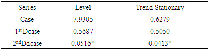
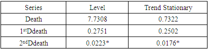
2.1. Unit Roots and Stationarity Tests: (Kwiatkowski-Phillips-Schmidt-Shin (KPSS) Test)

The KPSS test is a Unit root test that tests for the stationarity of a given series around a deterministic trend. It is used to test whether we have a deterministic trend or stochastic trend: KPSS test is conducted under the following hypothesis:

H₀: Y_t ~ I(0) trend stationary

H₁: Y_t ~ I(1) stochastic trend

If the null hypothesis is not rejected, it means that there is evidence that the series is trend stationary. The process is as follows:

Ø Regress y_t on a constant and time trend. Get Ordinary Least Square residuals

Ø Calculate the partial sum of the residuals:

(1)

Ø Compute the KPSS test statistic;

(2)

where is the estimate of the long-run variance of the residuals.

Ø Reject H₀ when KPSS is large

2.2. Nonlinearity and Structural Break Tests

The BDS and Tsay tests were adopted for testing nonlinearity in the series. The test of Brock et al. (1996) known as the BDS test, takes the concept of the correlation integral and transforms it into a formal test statistic which is asymptotically distributed as a standard normal variable under the null hypothesis of independent and identical distribution against an unspecified alternative Brooks C. (1996). Considering a time series x_t with h histories, , The correlation integral at embedding dimension h can be estimated by;

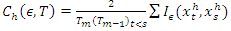(3)

where the parameter h is the embedding dimension, T is the sample size and is the maximum number of overlapping vectors that we can form with a sample of size T, is an indicator function that is equal to one if and equal to zero otherwise. A pair of vectors is said to be apart, if the maximum-norm is greater or equal to . Using this relation the BDS test statistic is defined as;

(4)

Where is the standard deviation of

The Tsay test of Tsay (1989), tests for evidence of threshold nonlinearity under the null hypothesis of linearity in the dataset. This test is an improvement of Keenan’s test for nonlinearity. Keenan (1985) proposes a nonlinearity test for time series that uses only and modifies the second step of the reset test to avoid multicollinearity between and . Tsay test improved on the Keenan’s test by allowing disaggregated nonlinear variables, that is all cross products of . Hence generalizing Keenan test by explicitly looking for quadratic serial dependence in the data.

The procedure is as follows;

Firstly, using any selection criterion, select the value p of the number of lags involved in the regression, then fit on to obtain the fitted values the residuals set and the residual sum of squares SSR. Then regress the product on to obtain the residual set The calculate;

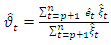(5)

The test statistics is the obtained as;

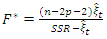(6)

This test statistic F^* is asymptotically distributed as where . Once there is evidence of nonlinearity, we proceed to check for the presence of structural break.

2.3. Unit Roots and Stationarity Tests

Kim and Perron, (2006) stated that in testing for unit root, it is necessary to consider the effects of structural breaks during unit root testing. Structural breaks play significant roles in that it can lead to misspecification of deterministic function of the auxiliary regression that is used for either testing for unit root or variance stationarity.

In this study, we consider the structural break unit root test of Zivot and Andrews (1992) and Perron (1989). Perron uses a modified Dickey-Fuller (DF) unit root tests that includes dummy variables to account for one known, or exogenous structural break. The break point of the trend function is fixed (exogenous) and chosen independently of the data. Perron’s (1989) unit root tests allows for a break under both the null and alternative hypothesis. These tests have less power than the standard DF type test when there is no break. However, Perron (1989) points out that they have a correct size asymptotically and is consistent whether there is a break or not. Moreover, they are invariant to the break parameters and thus their performance does not depend on the magnitude of the break. Zivot and Andrews (1992) endogenous structural break test is a sequential test which utilizes the full sample and uses a different dummy variable for each possible break date. The break date is selected where the t-statistic from the ADF test of unit root is at a minimum (most negative). Consequently, a break date will be chosen where the evidence is least favorable for the unit root null.

2.4. Markov Switching Vector Autoregressive Model Specification

The Markov Switching Model of Hamilton (1989), also known as the Regime Switching Model, is one of the most popular nonlinear time series models in the literature. This model involves multiple structures that can characterize the time series behaviors in different regimes or states or episodes. A novel feature of the Markov switching model is its Markovian property, which states that the probability of transitioning to any particular state is dependent solely on the current state, and not on the sequence of state that preceded it.

In this work we considered modeling the Markov Switching Autoregressive (MS-AR) process. We specifically consider a two regime-switching. We intend to model the regime S_t as the outcome of an unobserved 2-state Markov chain with S_t independent of v_t for all t. The MS-AR model for two regimes with autoregressive (AR) process of order k is as follows:

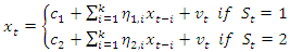(7)

Where the regimes are represented by The intercept and parameters of AR part are dependent of at time t. Given that we considered two regimes, we label regime 1 as representing the period of first wave of COVID-19 and we label regime 2 as representing the 2^nd wave of COVID-19. The transitions of the S_t are presumed to be ergodic and intricate 1st order Markov-process with transition probabilities

(8)

The transition matrix P captures the probability of switching, where;

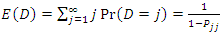
The nearer the probability is to one the longer it takes to shift to the next regime. The diagonal element of the matrix of the transition probabilities contains important information on the expected duration on the state of the regime.

Let D be defined as the duration of state j; we have:

(9)

(10)

Then the expected duration of regime j can be derived as;

(11)

As stated by Oluwasegun, A. A. et al (2020).

3. Results and Discussion

In this section, we present the results and discussion on the daily total infected cases and total deaths of COVID-19 data for Nigeria from 28^th February 2020 to 30^th September 2021.

3.1. Time Plot of the Series

A look at the time series plot of the total COVID-19 cases and deaths in Figure 1 shows that the total COVID-19 Cases and Deaths of Nigeria respectively has an upwards trend and is non-stationary.

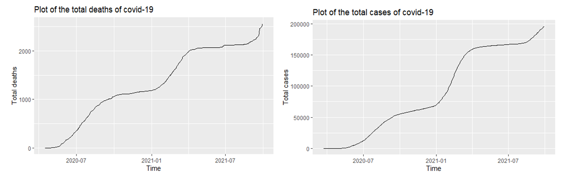Figure 1. Time series plot of the total COVID-19 cases and deaths of Nigeria

From Table 1, at 0.05 significance level, the 2^nd difference of the total cases is stationary while the original series and the 1^st difference of the original series are nonstationary.

Table 1. KPSS unit root test results based on total COVID-19 cases series

From Table 2, at 0.05 significance level, the 2^nd difference of the total deaths is stationary while the original series and the 1^st difference of the original series are nonstationary.

Table 2. KPSS unit root test results based on total COVID-19 deaths series

Figure 2 shows the time plots of the differenced series which strongly indicates evidence of non-stationarity, volatility clustering and change in structure hence we proceed to test for nonlinearity and structural break in the next sub section.

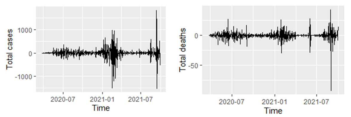Figure 2. Time series plot of the 2nd difference of the two series

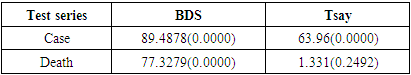
3.2. Nonlinearity and Structural Break Tests for the Returns

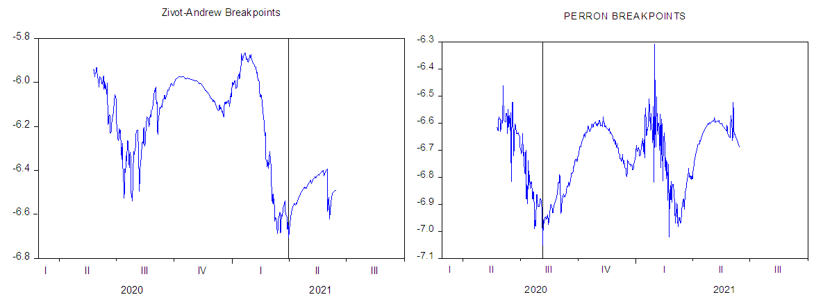
In this subsection, we present the results of the two nonlinearity tests. From Table 3, the results corresponding to the BDS and Tsay tests show that there is evidence of nonlinearity in both series. Furthermore, the Zivot-Andrew and the Perron breakpoint tests in Figure 3 and Figure 4 showed evidence of one structural break. The identified break dates are 30^th December, 2020 for Zivot-Andrew test, 6^th December, 2020 for Perron test each for the total COVID cases and for the total COVID deaths, 31^th March, 2021 and 5^th August, 2020 were the identified break dates from the Zivot-Andrew and Perron tests respectively.

Table 3. Nonlinearity test results

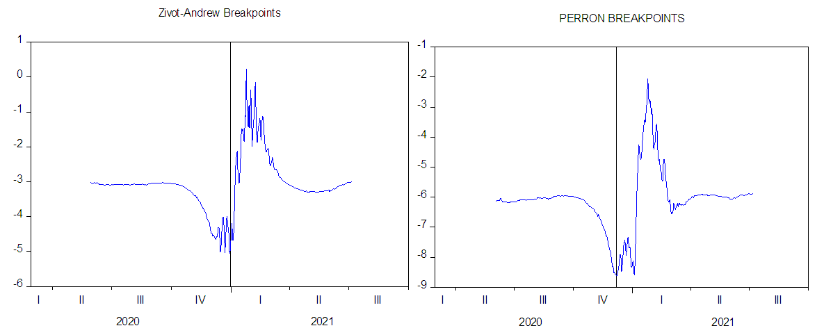Figure 3. Plot based on Zivot-Andrew and Perron test for the Total COVID-19 Cases

Figure 4. Plot based on Zivot-Andrew and Perron test for the Total COVID-19 Deaths

3.3. Model Estimation

The possible number of Covid-19 waves to be considered in the MSM model is determined on the basis of recursive local fitting as suggested in Gharleghi et al. (2014). The plot of the recursive residuals about the zero point, plus and minus two standard errors is shown in Figure 5.

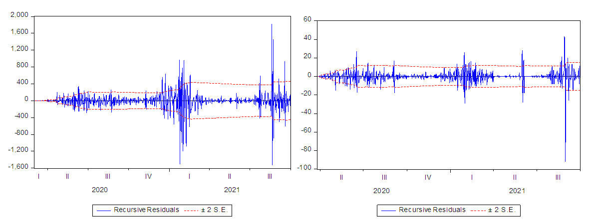Figure 5. Recursive Residual Plot for total infected cases and total death cases

The two figures above show that there is a significant wave change on the two occasions. Hence we proceed to fit a MSM(2)-AR(1) model for both the total infected cases and total death cases. The results of the fitted MSM(2)-AR(1) model is shown in the table below.

Table 4. The MSM(2)-AR(1) results for the Total COVID-19 Infected Cases

The table 4 above shows the estimated parameters of the infected cases. It shows that the expected number of cases for the 1^st wave rises by 297% daily, while that of the 2^nd wave rises by 118% daily. Also, the variance in 1^st wave is higher than that of the 2^nd wave which implies more volatile during the 1^st wave than during the 2^nd wave. This result high volatility of 1^st wave can be attributed to the period of the first total lockdown while the low volatility of 2^nd wave can be attributed to the period just before the end of the partial lockdown. Also, the expected duration for the 1^st wave was about 15 days while in the 2^nd wave it was about 52 days.

From table 5 the estimated parameters of the 1^st wave shows that the expected number of death rises by 7.1% daily while it rises by 1.7% during the 2^nd wave. Also, the variance in 1^st wave is higher than that of the 2^nd wave which implies that the total COVID-19 deaths is more volatile during the 1^st wave than during the 2^nd wave. This high volatility of the 1^st wave can be attributed to the period of the first total lockdown while the low volatility of the 2^nd wave can be attributed to the period just before the end of the partial lockdown. Also, the expected duration of 1^st wave was lower than that of the 2^nd wave, with about 46 days expected duration while for 2^nd wave its about 88 days.

Table 5. The MSM(2)-AR(1) results for the Total COVID-19 Deaths

The expected number of COVID-19 infected cases and Death cases matrix is given below;

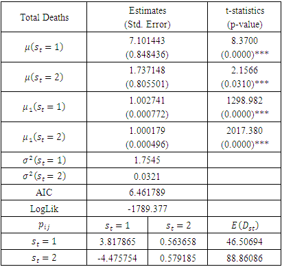
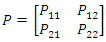
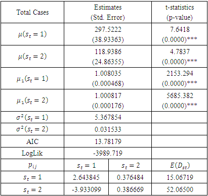
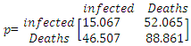And the transition probability matrix between the Expected numbers of COVID-19 infected

Cases and Death cases, is;

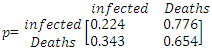This transition probability matrix can be used to predict the first, second, third periods etc. between the two waves for the number of COVID-19 infected and death cases.

4. Conclusions

This paper examined the nonlinear modelling of COVID-19 daily infected cases and deaths in Nigeria using the MS-AR model. The model estimates that the expected number of infected cases rises by 297% daily during the first wave of COVID-19 while it rises by 118% daily during the second wave of the pandemic. Also, the volatility of the two waves show that the COVID-19 infected cases in the first wave was more volatile than that of the second wave of the pandemic. The transition probabilities showed that in the first wave, the COVID-19 infected cases expected duration is around 15 days and 52 days in the second wave. For the COVID-19 deaths, the model estimates that the expected number of infected cases rises by 7.1% daily during the first wave of COVID-19 while it rises by 1.7% daily during the second wave of the pandemic. Also, the volatility of the two waves show that the COVID-19 infected cases in the first wave was more volatile than that in the second wave of the pandemic.