C. A. Igbo1, E. L. Otuonye2
1Department of Mathematics and Statistics, Federal Polytechnic Nekede, Owerri, Imo State
2Department of Statistics, Abia State University Uturu, Abia State
Correspondence to: C. A. Igbo, Department of Mathematics and Statistics, Federal Polytechnic Nekede, Owerri, Imo State.
| Email: |  |
Copyright © 2021 The Author(s). Published by Scientific & Academic Publishing.
This work is licensed under the Creative Commons Attribution International License (CC BY).
http://creativecommons.org/licenses/by/4.0/

Abstract
The square root transformation of the error component of the additive time series model was studied. The distribution of the transformed error component was established and shown that it is a proper probability density function. The properties of the distribution were investigated. It was shown that the mean of the transformed series  is equal to one while the mean of the original series = 0 for
  . Also, the variance of the transformed was established and given as
 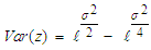 and is four times that of the original series for
  to one decimal place. The transformed series is normally distributed for
  .
.
Keywords:
Additive time series model, Square root transformation, Error component, Means, Variance, Left truncation
Cite this paper: C. A. Igbo, E. L. Otuonye, The Result of a Square Root Transformation on the Error Part of the Additive Time Series Model, American Journal of Mathematics and Statistics, Vol. 11 No. 4, 2021, pp. 73-93. doi: 10.5923/j.ajms.20211104.01.
1. Introduction
The normal distribution is a well known and most widely used in probability distribution. It is the most common distribution for independent randomly generated variables. The mathematical proof informed us that under certain condition, most distributions tend to the normal distribution. The normal distribution derives its usefulness from the famous Central Limit Theorem. (Hogg R.V and Graig, A.T, [1].The limits of the normal random variable X is  . However, there are situation where this random variable is constrained to be wholly positive or negative variables. This will now force us to study the behavior of the random variable under these restricted conditions. A typical illustration of this is the study of error part of the model. Its square root is constrained to positive values only. Iwueze [2] established the distribution of the truncated normal distribution and is given by;
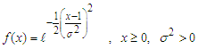 with mean E(x) and variance, Var(x) given by;
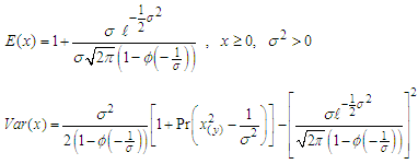 In the work, the implication of truncating the
  to the left was investigated. The distribution of the error part of the multiplicative time series model is given by
  .Okoroafor et al [3] studied the method of handling transformations of the error component when the time series model is additive that is
  . In the work, he detailed the effect of truncating the normal distribution of the irregular component of the additive model and established the condition for a successful transformation. The mean and variance were derived and expressed as:
  and
and 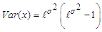 .Time series is a well arranged set of data that occur sequentially over time. However, the Trend
  , Seasonal
  , Cyclical
  and error
  are the components of time series. The trend and the cyclical components are usually combined to give the trend-cycle component especially in a short term series Chatfield [4].For short time series especially, we have three mostly used models in the analysis of descriptive time series. Multiplicative;
  Additive;
 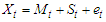 Mixed;
  Where,
  is a combination of Trend
  and Cyclical
  . components.Data Transformation: this is a mathematical tool used in converting data from one structure to another. In addition to stabilization of variance, it reduces the variance of the variable and ensures a normally distributed data and additivity of the seasonal effect. It can also be used to (a) Ensue better organization and give easier and more appropriate utilization.(b) It improves the quality of the data and in certain cases, reduces the error committed if not transformed.There are several statistical literatures on the effects of transformations on the error component of the multiplicative time series model. Most of the work centered on establishing the condition under which the transformation would be successful and fulfill the purpose for such transformation. A transformation is successfully achieved when the conditions of the original series are not significantly altered.Iwueze (2) studied the
  distribution when the values do not admit values less than zero. He showed that the truncated values are greater than zero if and only if
  . He showed that the mean of the left truncated
  distribution is in terms of the cumulative distribution of the standard normal distribution while that of variance is in terms of the chi-square distribution with one degree of freedom.Akpanta and Iwueze [5] investigated the effect of the logarithmic transformation on the seasonal and trend-cycle components of the multiplicative time series model. They obtained intervals within which the required seasonal indices of a purely multiplicative time series model would lie for a successful logarithmic transformation.Iwu et al [6] studied the effect of the six transformations (logarithmic, square, square root, inverse, inverse square root and inverse square) on the trend-cycle
  and seasonal
  components of the multiplicative time series. Bond and Fox [7] gave genuine reasons for adopting data transformation such as improvement of normality, stability of variance and conversion of scales to interval measurements.Osborne [8] opined that data transformation are the application of a mathematical modification to the values of the variable and expressed that caution should be exercised in the choice of the type of data transformation to be adopted so that the fundamental structure of the series is not distorted and thereby rendering the interpretation difficult or intractable.Iwueze and Nwogu [9] studied the relationship between the periodic mean and variance and showed a plot of the periodic mean and standard could determine the appropriate model to adopt in the analysis of time series model.
2. Methodology
In this work, we are interested in the properties of the square root transformation of the additive time model as against the multiplicative which has been extensively studied Hence, the following would be carried out;(a) The probability density function of the square root transform of the error component would be derived and thereafter show that it is a proper probability density function.(b) Establish the mean and variance of the distribution and see how it effectively compares with the mean and variance of the original series.(c) The use of simulation would be used to see how the theoretical mean and variance compares with the simulated values.(d) To find out if the square root transformation conforms to the normality assumption of the original series under specified condition.(e) To investigate whether the square root transformation of the additive model compares favorably with the square root transformation of the multiplicative model.
3. Results
3.1. We Would First Find the Probability Density Function of the Square Root Transformation of the Error Component of the Additive Model
Let z be the transformed variable while y is the error variable. The probability density function of the truncated variable according to Okoroafor et al (3) is given by; 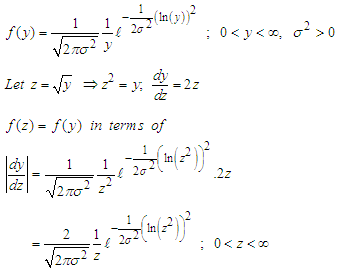 Simplifying further, we have
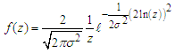
3.2. We Now Show that It is a Proper PDF. For a Proper PDF, We have That
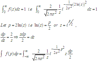 Where the limit of p is
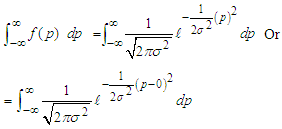 This is the probability density of a normal distribution with mean 0 and the variance
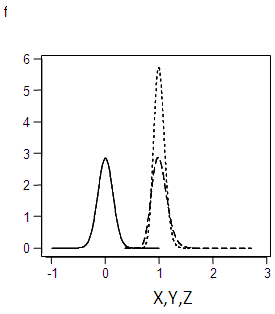
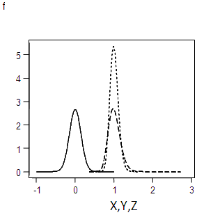
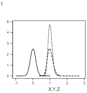
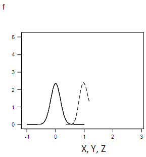
  whose integral within the limits = 1.The graph forms of the square root transformed data for the specified values of σ are shown in appendix 1.
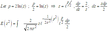
3.3. We then Find the 
 the limits of p =
 By completing the square we have
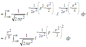 But
But 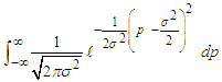 is the pdf of
  whose integral within the limits = 1.
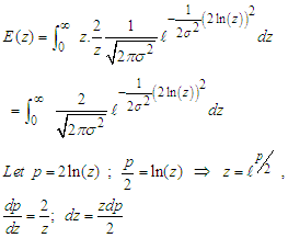
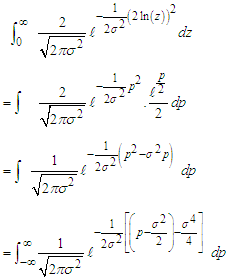
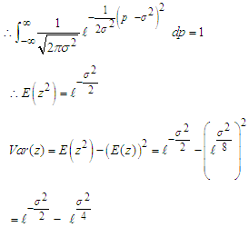
3.4. Variance of z: Var(z)
 By substituting for z and simplifying, we have
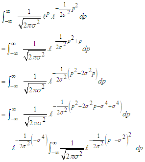 That is by completion of square
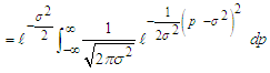 But
But 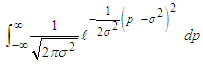 is the pdf of
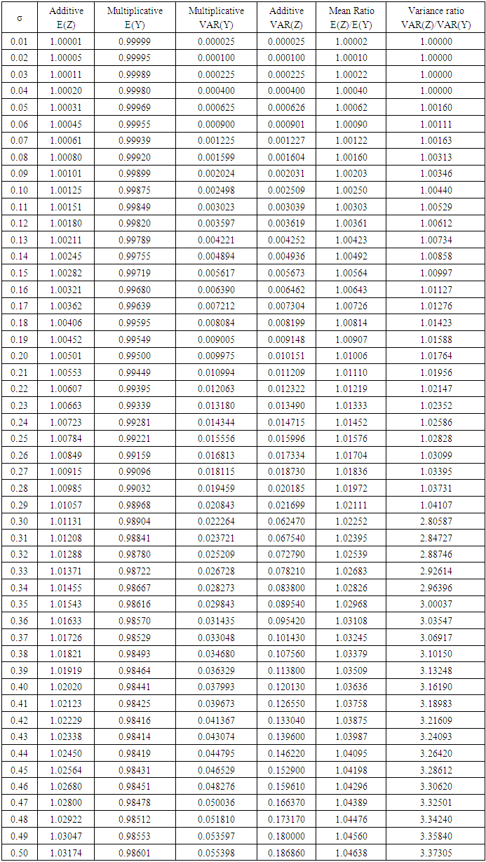
3.5. The Mean and Variance of the the Original Series and Square Root Transformed Series are Shown in Table 1 for 0 ≤ σ ≤ 0.5
Table 1. Comparison of means and variances
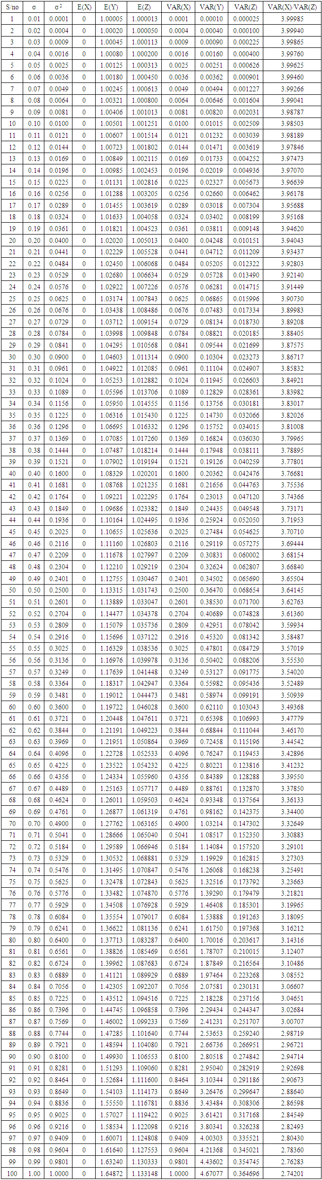 |
| |
|
The comparison of the means and variances is shown in table 2.1.Table 2.1. Comparison of the means and variances
 |
| |
|
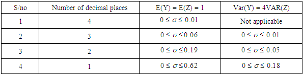
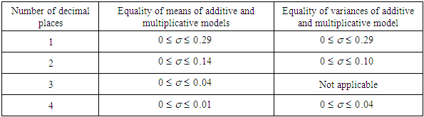
Depending on the level of accuracy demanded, we have the following conditions for the mean of the transformed to be equal to 1.0 and variance of the original series is equal to 4 times the variance of the square root transformed series as shown in table 2.1 above.The abridged comparison of the means and variances of the multiplicative and additive models are shown in appendix 4. The condition under which the means and variances of the additive and multiplicative multiplicative models are equal is as given on table 2.2.Table 2.2. Summary of the comparison of the means and variances of the additive and multiplicative
 |
| |
|
From table 2.2, it is seen that for  the means and variances of the two models are the same to one decimal place.
3.6. Simulated Examples
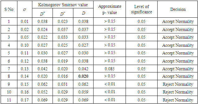
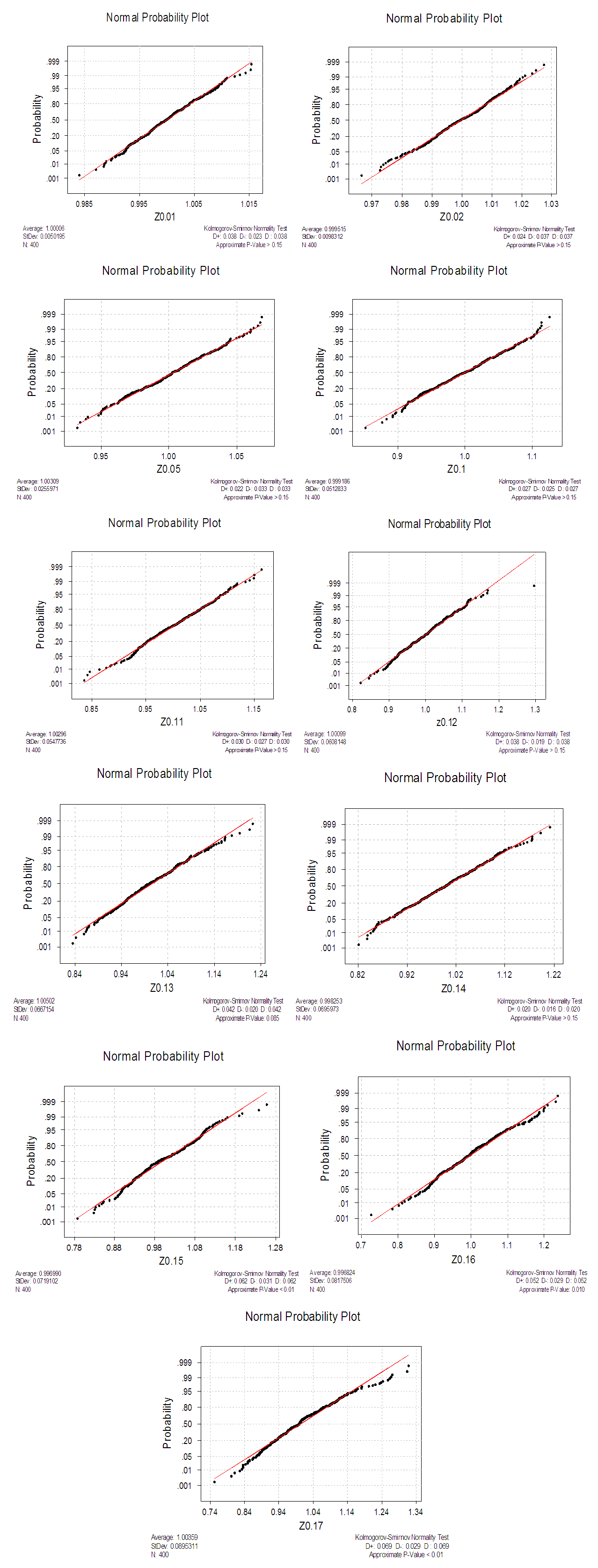
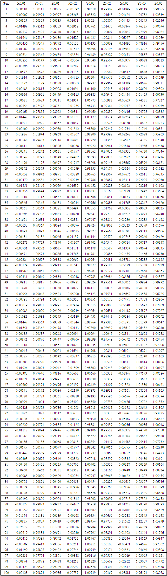
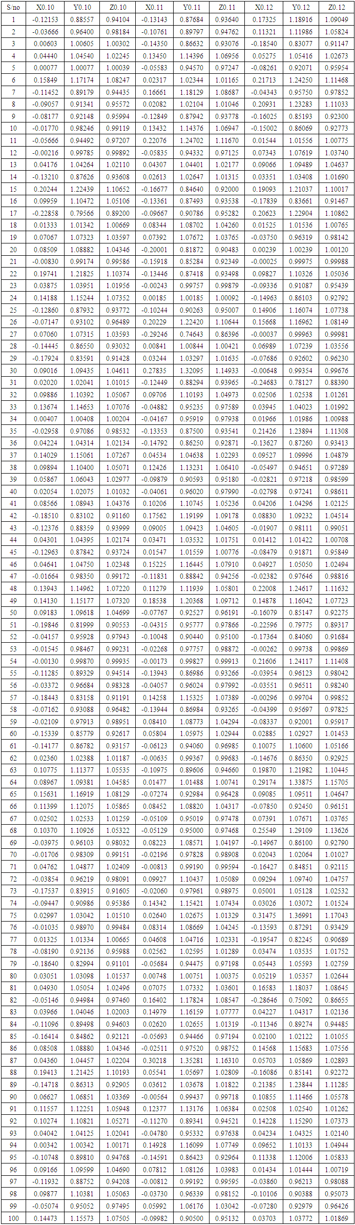
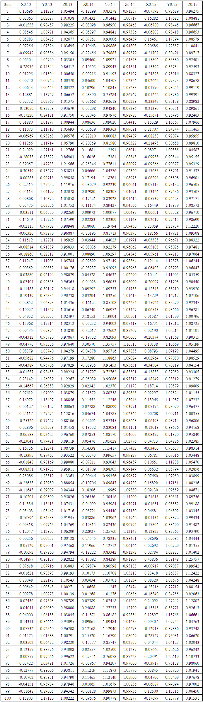
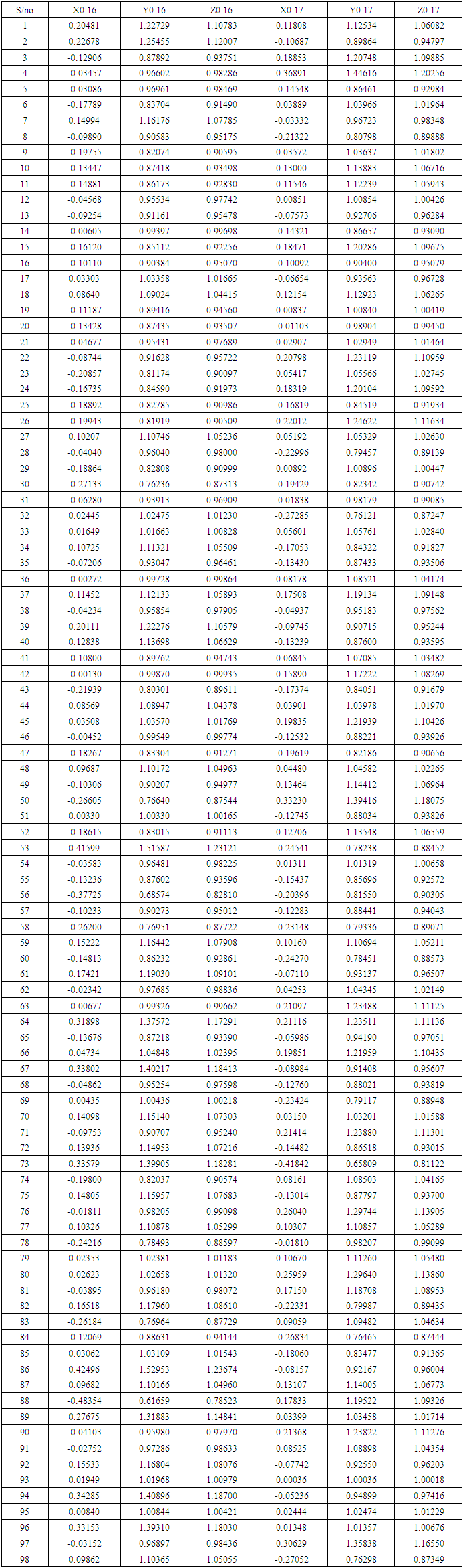
Simulations using Minitab were carried out for values of Z with mean 0 and various values of the standard deviation. For want of space, only simulations of some values of σ were shown. A summary of the analysis of the simulated values mentioned above is however presented on table 2. The corresponding values of the transformed series were obtained for σ = 0.01, 0.02, 0.03, 0.05, 0.1, 0.11, 0.12, 0.13, 0.14, 0.15, 0.16 and 0.17. A summary of the analysis of the simulated values mentioned above is however presented in appendix 2. Also in this section, considering that the original distribution is  , we would also test for the normality of the square root distribution using Kolmogorov-Smirnov Goodness-of-Fit test (One sample case).
3.7. Test of Normality
A summary of the test of normality of the square root transformed series is shown on table 3 for specified values of  .
.Table 3. Summary of Kolmogorov-Smirnov Test of Normality for the transformed series (For the specified values of σ)
 |
| |
|
4. Summary and Conclusions
a) The probability density function of the square root transformed error component of the additive time series model was established and shown to be 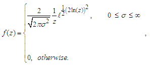 b) It was also proved that it is a proper probability density function as shown in 3.2. The graph forms of the probability density function for the specified values of
  were shown in appendix 1. The comparative analysis of the mean and variances was carried out for
  to four decimal places and shown in table 1 c) The mean and variance of the distribution was shown on 3.3 and 3.4 to be
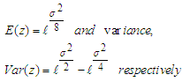 d) The Kolmogorov Smirnov test of normality for the transformed series was carried out and summarized on …. It was shown that the series was normal for
  . Therefore, for the structure of normality of the original series not to be violated, all inferences on the transformed series should be done within this value of
  e) From table 2.2, it is seen that for
  the means and variances of the two models are the same to one decimal place.
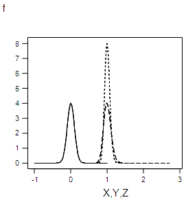
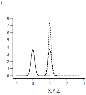
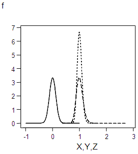
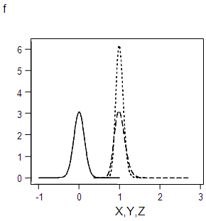
Appendix 1: Graph Forms of the Original, Truncated and Square Root Transformed Series for the Specified Values of σ
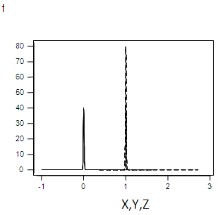 | Figure 3.1. Graph of f(x), f(y), f(z) for α=0.01 |
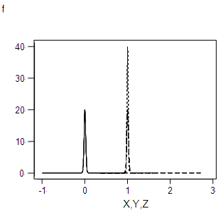 | Figure 3.2. Graph of f(x), f(y),f(z) for α=0.02 |
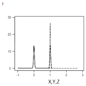 | Figure 3.3. Graph of f(x), f(y),f(z) for α=0.03 |
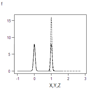 | Figure 3.4. Graph of f(x), f(y),f(z) for α=0.05 |
 | Figure 3.5. Graph of f(x), f(y),f(z) for α=0.1 |
 | Figure 3.6. Graph of f(x), f(y),f(z) for α=0.11 |
 | Figure 3.7. Graph of f(x), f(y),f(z) for α=0.12 |
 | Figure 3.8. Graph of f(x), f(y),f(z) for α=0.13 |
 | Figure 3.9. Graph of f(x), f(y),f(z) for α=0.14 |
 | Figure 3.10. Graph of f(x), f(y),f(z) for α=0.15 |
 | Figure 3.11. Graph of f(x), f(y),f(z) for α=0.16 |
 | Figure 3.12. Graph of f(x), f(y),f(z) for α=0.17 |
Appendix 2: Kolmogorov-Smirnov Test of Normality for the Transformed Series (for Specified Values of σ)
 | Appendix 2. Kolmogorov-Smirnov Test of Normality for the Transformed Series (for Specified Values of σ) |
Appendix 3: Simulated Values of Originl, Truncated and Square Root Series
Appendix 3. Simulated Values of Originl, Truncated and Square Root Series
 |
| |
|
Appendix 3. Continue
 |
| |
|
Appendix 3. Continue
 |
| |
|
Appendix 3. Continue
 |
| |
|
Appendix 4: Comparative Analysis of the Means and Variances of the Square Root Transformations of the Additive and Multiplicative Models
Appendix 4. Comparative Analysis of the Means and Variances of the Square Root Transformations of the Additive and Multiplicative Models
 |
| |
|
References
| [1] | Hogg. R. V. and Craig, A. T. (1978). Introduction to Mathematical Statistics. 4th ed., Macmillan Publishing Company, New York. |
| [2] | Iwueze, I. S. (2007), Some Implications of Truncating the  Distribution to the Left at Zero. Journal of Applied Sciences (7)2; 189 – 195. Distribution to the Left at Zero. Journal of Applied Sciences (7)2; 189 – 195. |
| [3] | I B Okoroafor, E.L Otuonye, D.C Chikezie, and A.C Akpanta (2021), Method of Handling Transformation when the Time Series Model is Additive, Advanced Journal of Statistics and Probability (9)1 pp17-31. |
| [4] | Chatfield, C. (1980). The Analysis of Time Series: Theory and Practice, Chapman and Hall, London. |
| [5] | Iwueze, I. S. and Akpanta A. C. (2007). Effect of the logarithmic transformation on the trend-cycle component of the multiplicative Time series Model. Journal of Applied Sciences. (7)17, 2414-2422. |
| [6] | Iwu H.C, Iwueze I.S, and Nwogu E.C (2009), Trend Analysis of Transformations of the Multiplicative Time Series Model, Journal of the Nigerian Statistical Association, Volume (21)5, pp 40-54. |
| [7] | Box, G. E. P. and Cox, D. R. (1964), Analysis of Transformations. J. Roy Statistics Society B – 26, 211 – 243, discussion 244 – 252. |
| [8] | Osborne, J. (2002), Notes on the Use of Data Transformations, J. Practice Practical Assessment, Research and Evaluation, 8 (6). |
| [9] | Iwueze I S and E C Nwogu (2004), Buys-Ballot Estimates for Time Series Decomposition, Global Journal of Mathematical Sciences, Vol.(3)2, pp83-98. |
| [10] | Otuonye, E. L., Iwueze, I. S. and Ohakwe, J. (2011), The Effect of Square Root Transformation on the Error Component of the Multiplicative Time Series Model,. International Journal of Statistics and Systems. (6)4; 461 – 476. |

 Abstract
 Reference
 Full-Text PDF
 Full-text HTML