-
Paper Information
- Paper Submission
-
Journal Information
- About This Journal
- Editorial Board
- Current Issue
- Archive
- Author Guidelines
- Contact Us
American Journal of Mathematics and Statistics
p-ISSN: 2162-948X e-ISSN: 2162-8475
2021; 11(3): 61-66
doi:10.5923/j.ajms.20211103.02
Received: Apr. 4, 2021; Accepted: May 7, 2021; Published: May 26, 2021

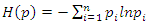
Maximum Entropy Estimation: Agronomic Dataset
 Abstract
 Reference
 Full-Text PDF
 Full-text HTML
Raymond Bangura1, Sydney Johnson2
1Biometric Unit, Sierra Leone Agricultural Research Institute, Freetown, Sierra Leone
2Department Agronomy, Rokupr Agricultural Research Center, Kambia District, Sierra Leone
Correspondence to: Raymond Bangura, Biometric Unit, Sierra Leone Agricultural Research Institute, Freetown, Sierra Leone.
| Email: |  |
Copyright © 2021 The Author(s). Published by Scientific & Academic Publishing.
This work is licensed under the Creative Commons Attribution International License (CC BY).
http://creativecommons.org/licenses/by/4.0/

We provide a generalized maximum entropy method and its application to the Agronomic dataset. Errors of deviation are shown with the analysis of variance on the entropy method. Multi-collinearity is one of the major problems of regression analysis. Based on the maximum entropy method, we gave a better estimate than the traditional robust regression of four independent variables from an Agronomic dataset. From the generalized maximum entropy method, we showed the relationship between the dependent and independent variables. Also, we provided a diagnostic fit for the dependent variable to support the theoretical analysis.
Keywords: General maximum entropy, Multicollinearity, Support space, Regression, Residual
Cite this paper: Raymond Bangura, Sydney Johnson, Maximum Entropy Estimation: Agronomic Dataset, American Journal of Mathematics and Statistics, Vol. 11 No. 3, 2021, pp. 61-66. doi: 10.5923/j.ajms.20211103.02.
Article Outline
1. Introduction
- The maximum entropy method has gained a spectrum of recognition in many disciplines, such as Mathematics, Engineering sciences, and statistics. The maximum entropy principle was proposed by Shannon, 1948, which states that an inference is made based on incomplete information draws from the probability distributions that maximizes the entropy that is subject to constraints on the distribution. In order words, when given a large number of probability distributions, we choose the one that best represents the present state. The process of choosing the highest uncertainty is known as the maximum entropy. There are infinite number of possible models that satisfy the constraints (Simon Haykin, pg481). As a result of this, the maximum entropy is a constrained optimization technique. The maximum entropy includes numerical solutions of stationary density functions by Perron-Frobenius operator, introduced by J. Ding 1995 in the study of dynamic systems. A generalized maximum entropy estimator is a robust estimator that resists multicollinearity problems. The maximum entropy estimates the parameters in a linear regression model, especially when the data are ill-posed. The generalized maximum entropy estimator has played a vital role in the econometric model estimation because it is an alternative estimator to least squares (Wilawan Srichaikul, 2018). Akdeniz et al., 2011, provided an alternative estimation method of maximum entropy to estimate parameters in a linear regression model especially when the basic data are ill-conditioned. The generalized maximum entropy helps find information about variables or measures through probability functions using the Shannon method of general maximum entropy. Based on the generalized maximum entropy method, Bangura et al., 2020, provided a good estimate of three variables from a rice seed data. To this present moment, the estimation of parameters by the maximum entropy method is still rare because regression analyses are posing with threat of multi-collinearity and ill-conditioned dataset. The primary task in using the GME approach as an estimator to choose an appropriate entropy measure that reflects the uncertainty (state of knowledge) that we have about the occurrence of a collection of events (Wilawan Srichaikul, 2018). The paper also estimates the value of the generalized maximum entropy residuals of the weighted variables, which quantifies the amount of information in a variable, providing the basis for an assumption about the concept of information derived from the variables (weighted). We also found a linear regression from the generalized maximum entropy procedure to show the relationship between endogenous (explained variable) and exogenous (regressors) because a generalized maximum entropy estimator is a robust estimator that is strictly resistant to multicollinearity.In this paper, we considered four parametric variables are; panicle (Pan), plant height (Plant_Ht), panicle length (Pan_Length), and Tillers (dependent) taken from the data set in 2014 and 2015. The paper is divided into five sections. We introduced the topic in section one. In section we gave the theoretical background of the maximum entropy method followed by its application in section three. We examined the residuals in section four and gave our conclusion in section five.
2. Generalized Maximum Entropy
- Jaynes (1957) proposed the method of maximizing entropy by recovering unknown probabilities by characterize dataset, subject to the available sample moment information, and adding up constraints on the probabilities (Simon Haykin, pg481).
 Linear Constraint
 For
For  Within the classic ME framework, the observed moments are assumed to be exact. To extend this approach to the problem with noise, the GME approach (developed by Golan, Judge, and Miller (1996)) generalizes the ME approach by using a dual objective (precision and prediction) function.The generalized maximum is the covariance estimate shows 596 convergence criteria. It gives the estimate of four parameters. From the classical general linear model (GLM), we have;
 | (1) |
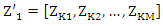 and the vector of probabilities associated with the M dimension is given as
 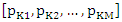 Now, we can rewrite matrix form as;
 | (2) |
 and
and  from (2) in such a way that they both represent probabilities accordingly. That is;
 So we have; under this re-parameterization, the inverse problem with noise given in (1) may be rewritten as
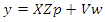 | (3) |
 is the
  known matrix of explanatory variables and
  is a
is a  noise (disturbance) vector.According to Golan, 1996 we aim to convert each parameter
  If
If  with an equal distance discrete support values,
  with corresponding probabilities
  By this way, each parameter is converted from the real line into a well-behaved set of proper probabilities defined over the supports.
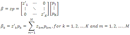 Also, the disturbance (noise)
  with assign probabilities
 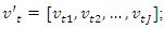 given that
  We have;
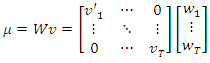 Likewise;
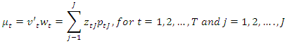 As for the determination of support bounds for disturbances, Golan et al (1996) recommend using the “three-sigma rule” of Pukelsheim (1994) to establish bounds on the error components: the lower bound is
  and the upper bound is
  , where σy is the (empirical) standard deviation of the sample y. For example if J= 5, then
 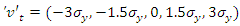 can be used.Jaynes (1957) demonstrates that entropy is additive for independent sources of uncertainty. Therefore, assuming the unknown weights on the parameter and the noise supports for the linear regression model are independent, we can jointly recover the unknown parameters and disturbances (noises or errors) by solving the constrained optimization problem of max;
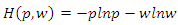 Subject to
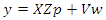 When
When  and
and  are re-parameterized, and are transformed with assigned probabilities.
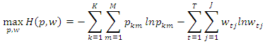 Constraints
 By solving the first order condition, the estimates of the GME parameters are given by;
3. Generalized Maximum Entropy Application
3.1. Final Information Measures
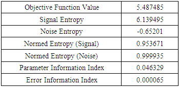
- Table 1 shows the final information summary as assumed that the information is incomplete in estimating the generalized maximum entropy. The objective function value includes prediction and precision given at 5.49. The objective value function represents the value of the entropy estimation problem. The signal entropy is 6.14, noise is -0.65, normed (signal) is 0.95, normed (noise) is 0.99, parameter information index is 0.046 and the index information error is given as. It implies that the dataset is viable for analysis because the value of error-index information is too low.
|
|

3.2. Generalized Maximum Entropy Variable Estimates
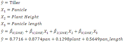
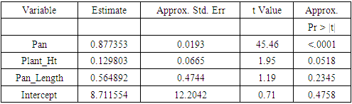
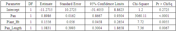
- Table 3 provides the estimate of the generalized maximum entropy method of three parameters. It shows that the panicle is highly significant at 5% with a high influence on the estimated response (tiller) than the other independent variables. Also, Table gives a better estimate of the parameters than the robust regression in Table 4.1.
|
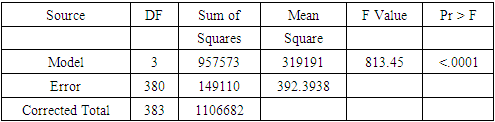
3.3. Analysis of Variance
- Table 4 shows the analysis of variance for the three independent variables which are; panicle, plant height and panicle length. It shows that they are highly significant at

|
4. Residuals
- Figure 1 shows the residuals versus observation number. It shows that the deviation values are concentrated within the range -2 to +2. We see that most of the points lie close to zero and they are relatively homogeneous. Figure 1 also provides the regression model for the four variables and their relationship with the dependent variable. Figure 1 also shows an entropy regression, which is quite different from the generalized maximum entropy estimate. It shows the coefficient of determination is 0.8642 and root mean square error is 19.809. In table 5, we ran a robust regression to reduce outliers by finding a shrinkage estimator with the presence of two outliers.

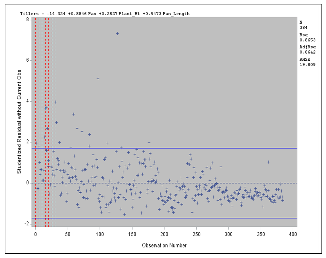 | Figure 1. Showing residuals and observation points |

|
4.1. Fit Diagnostics for Dependent Variable (Weights)
- Figure 2 shows that the regression is good as most points are not too far from the regression line with a good precision. The predicted value plot and the quantile plot depict a partially extreme value fit because they are almost linearly related. In figure 2, the diagnostic fit has no adequacy or validity threats to the dependent variable (Tiller).
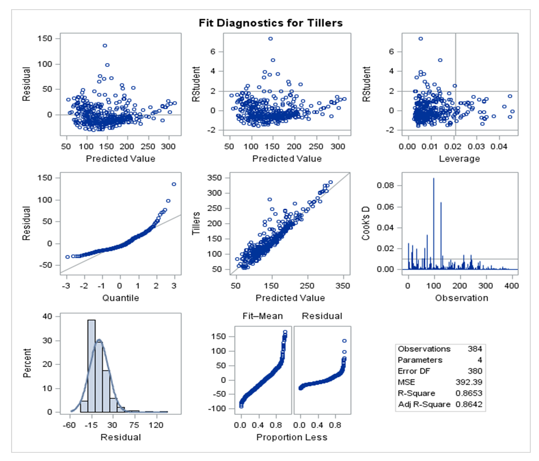 | Figure 2. Diagnostics fit for Tillers |
5. Conclusions
- We have applied the generalized maximum entropy method for the estimation of four Agronomic variables. The result from the analysis shows that the GME-estimates differ from the robust regression-estimate in their intercepts. So, the maximum entropy provided a better estimate of these variables than the robust regression. In the model, panicle influence is high on the tiller than the other independent variables. We also found out that the panicle is highly significant at 5 percent from the analysis of variance and we detected two outliers from the residual analysis.
ACKNOWLEDGEMENTS
- We appreciate the Sierra Leone Agricultural Research Institute for providing the research fields and part funding. We also thank Seibersdorf Laboratories for providing both radiation sources for rice varieties and the International Atomic Energy Agency (IAEA).