Benson Ediri Uwhowho , Happiness Onyebuchi Obiora-Ilouno
Department of Statistics, Nnamdi Azikiwe University, Awka, Nigeria
Correspondence to: Benson Ediri Uwhowho , Department of Statistics, Nnamdi Azikiwe University, Awka, Nigeria.
| Email: |  |
Copyright © 2021 The Author(s). Published by Scientific & Academic Publishing.
This work is licensed under the Creative Commons Attribution International License (CC BY).
http://creativecommons.org/licenses/by/4.0/

Abstract
In this paper, twenty gamblers were examined. Their lottery activities in the Golden Chance Lotto in Ekakpamre Community were recorded for the period of 30 days. It was clearly observed from the study that lotteries have an extremely low probability of winning. Using Chapman Kolmogorov equation, a transition probability matrix was established which described the game. The probabilities generated from the lottery records revealed that the chance that a lottery player would win and win again is 0.21818182 whereas the probability that the same player would lose and lose again is 0.9180952. This explains the reason for the high losses incurred by lottery players no matter how hard they try. The 5 out of 90 lottery carries a one in 44 million probability of winning the jackpot. Thus if all the possible numbers are listed out, the only way one could be sure of having a win is to get as many as 44 million people who will each play one of the number combinations. In this case one person wins the jackpot but 43999999 persons lose. Definitely, this is not a wise venture. If a player plays a lottery (Golden Chance Lotto) five times daily, it will take approximately twenty four thousand and eighty two (24081.79) years to hit the jackpot. An almost impossible situation. With an extremely low probability of winning and the very low payout ratio, buying lotteries is evidently a losing proposition. Obviously, the house (that is the lottery company) always wins why the gambler loses at all times as the payout money at any point is part of the losses of other gamblers.
Keywords:
Lottery, Probability, Transition, Jackpot
Cite this paper: Benson Ediri Uwhowho , Happiness Onyebuchi Obiora-Ilouno , The Probability of Winning a Lottery Game (A Case Study of Golden Chance Lotto, Ekakpamre Community, Ughelli South Local Government of Delta State), American Journal of Mathematics and Statistics, Vol. 11 No. 2, 2021, pp. 34-40. doi: 10.5923/j.ajms.20211102.02.
1. Introduction
The drawing of lots to determine ownership or other rights is recorded in many ancient documents. A lottery is a game that is used to raise money. At its most basic level, a lottery involves paying a small amount of money to purchase a ticket for the chance to win a prize, such as a large sum of money. Lotteries don't involve skill, since lotteries are determined purely by chance. There are many different types of lotteries: from simple 50/50 drawings at local events where the winner gets fifty percent of the proceeds from tickets sold to multi-state lotteries with jackpots of several million Naira. Casting of lots to clear situations of doubt or to find out some hidden facts could be traced to bible days. However casting of lots as it was used in bible days was purely for decision making which could be related to simple random sampling today and table of random numbers. This is quite different from how it is being used as lottery today.Golden Chance Lotto is a game of numbers which involves 1 to 90 numbers, whereby only the first five drawn numbers are considered as the winning numbers, and being paid for. Bet is rewarded according to the amount and the factor placed on each. For 2 direct the factor is N240, which will be multiplied by the amount played (staked) with. 3 direct has factor of N2,100, 4 Direct has factor of N4,000 and 5 direct is factor of N75,000. Direct, permutation, and against are the betting system adopted. “The bigger the risk, the higher the amount to be won”. The betting system adopted are as follows.(i) DIRECT: This is when you select 2 numbers and place bets on it. If the 2 selected numbers comes out amongst the five winning numbers, the bet is won. It can be done for 3, 4 and 5 also using the above factors.(ii) PERMUTATION: This is when you select more than 2 numbers and predict that, at least two of the selected numbers will drop amongst the winning numbers. The selected numbers can be between 3 and 10. i.e. Perm 2 from 10 numbers.(iii) AGAINST: This is when you select 1 or more numbers to bet with some sets of numbers, where the selected number must come out with at least one of the set of numbers, amongst the winning numbers.Clotfelter and Cook (1989) noted that lottery associations encourage conscious selection in marketing related to their products perhaps to increase demand by players who wish to “control their destiny.” Conscious selection also reduces the coverage of number combinations in any given draw, increasing the probability that a jackpot prize will roll over and potentially attracting additional sales in future draws in response to the higher advertised jackpots.Grote and Matheson (2006) observed that although state-operated lotto games have the worst average expected payoffs among common games of chance, because the jackpot can accumulate, the maximum expected payoff is potentially unlimited. It is possible; therefore, that lotto can exhibit a positive expected return. They examined 18,000 drawings in 34 American lotteries and found approximately 1% of these drawings provided players with a fair bet and further stated that, if it were possible for a bettor to purchase every possible combination, most lotteries commonly experience circumstances where such a purchase would provide a positive return with 11% of the drawings providing a fair bet to the player.Clotfelter and Cook (1991) observed that gamblers tend to withdraw their bet on certain numbers after such numbers hit the jackpot. This is owned to the fact that gamblers believed that the probability of drawing a number again after it had hit the jackpot is reduced for several weeks or months. As a result of this fallacious perception, players who ordinarily favour such numbers will either switch to another number or stop playing for a while. They further explained that gambler’s fallacy is the belief that the probability of an event is lowered when the event has recently occurred, even though the probability of the event is objectively known to be independent from trial to trial.Burger et al. (2003) introduced the novel notion of a lottery graph, derived some of its properties and demonstrated how standard results from graph domination theory, not previously associated with the lottery problem, lead to simple, closed-form analytic bound formulations for the lottery number. They developed a search procedure for characterizing all possible overlapping structures of sets used to establish 19 new lottery numbers and to improve upon best known bounds for a further 20 lottery numbers.Kucharski (2016) almost appears to unveil the well-guarded secret that mathematics can make gambling profitable, turning it into a real profession of a kind on the other hand, such a professional secret comes with a cold warning that while exploiting mathematics in gambling may sometimes lead to huge profits, the path to becoming a successful gambler is difficult. He then approaches a central question: can one actually exploit scientific knowledge for success in gambling? The answer depends on the game in question, of course, but if the answer is yes, the edge between gambling and games of pure skill, such as chess, grows thinner.Barnes et al. (2011) examined the prevalence and socio-demographic correlation of gambling and problem gambling across the lifespan and focused specifically on gambling on the lottery which is the most prevalent form of gambling in the United States and discovered that the frequency of gambling on the lottery increased sharply from mid adolescence to age 18 which is the legal age to purchase lottery tickets in most states. They observed that lottery play continued to increase into the thirties when it leveled off and remained high through the sixties and then decreased among those 70 years and above. They also considered multiple socio-demographic factors together in a negative binomial regression and found that the average number of days of lottery gambling was significantly predicted by male gender, age, neighborhood disadvantage and whether or not lottery was legal in the state where the respondent lived.Beckert and Lutter (2008) examined the distribution effects state lotteries have on Germany's social structure and noted that lotteries are highly taxed economic transactions, whose proceeds make up a considerable share of public fiscal revenues. Their analysis showed that lotteries are a form of regressive taxation, using key demographic indicators, such as age, citizenship, and levels of income and education, demonstrated the effects of fiscal redistribution.Keen, Anjoul and Blaszczynski (2019) explained that educational programs may be conceived as a demand reduction strategy by encouraging informed decision making among individuals. However, such education competes against the overwhelming volume of advertisements from the gambling industry encouraging people to gamble regularly as well as easy access to many gambling opportunities. The purpose of educational programs may be better conceptualized as promoting informed choice in line with a suite of broader preventative measures including regulation, legislation, and key stakeholder responsibilities.Ashong (2020) said that a lotto operator was fined by the National Lottery Regulatory Commission for failing to pay its winners. Sponge Nigeria Limited was fined N10million by NLRC for failing to pay monies amounting N138million to its winners in its last promo titled, ‘Better Life Billionaire Promo’. The company was also directed to pay the monies without any further delay or face the consequences which may be severe.Doll (2012) collected the true, terribly sad stories of lotto winners that showed that winning the lottery, despite the seeming wonderfulness of having some $600-million more dollars (before taxes) to your name, is not all it's cracked up to be. He said that in fact, what seems like an American dream may actually be something of an American nightmare.From the literatures studied, it observed that a transition probability matrix had not be derived to describe the lottery game and the probability of winning or losing Golden Chance Lotto in particular had not been studied. Thus this paper aimed to estimate the probability of winning or losing in a Golden Chance Lotto game with the view to establishing the true state of players in a particular game, to establish a transition probability matrix for describing the game based on the data collected, to compare the probability of winning and winning again to that of losing and losing again using Chapman Kolmogorov equation to establish an n-step probability matrix for the players and to calculate the probability of hitting the jackpot in Golden Chance Lotto Game and the time it may take to hit a jackpot.
2. Methodology
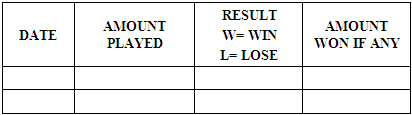
In order to know the probability of winning a lottery game, a particular lottery company (Golden Chance Lotto) was selected out of the numerous lottery companies in Nigeria. The Golden Chance Lotto is a lottery company that is present in almost every community in Nigeria and therefore provided a good platform for the research. Primary data were collected from 25 gamblers from the ages of 20 to 60 who volunteered their daily lottery records. A gambler here is defined as someone who plays the Golden chance lotto at least once a day. Table 1. A sample of the questionnaire used for data collection
 |
| |
|
The questionnaire was made up of four columns as shown in table 1 above. The amount used for the gambling was recorded. At the end when the result of that particular game is out, the player checks if he wins or loses and W or L is entered for win or lose respectively. If he wins the amount won may be recorded. A total period of 30 days was allocated to each participant/respondent for the data collection. A transition probability matrix was developed from the data to describe the game by each of the gambler. The data were analyzed using statistical software R program.
2.1. Chapman-Kolmogorov Equations
The n-step transition probability that a process currently in state  will be in state j after n additional transitions can be very useful in estimating the probability at any given step and is written as:
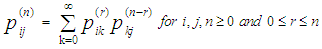 | (1) |
Note that 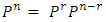 This equation shows that going from state
  to j in n-steps, the process will be in some state k after exactly
  steps. In essence the
  is just the conditional probability that starting from state i, the process goes to state k after r steps and then to state j in n-r steps. When we sum the conditional probabilities over all possible states we must get
  .Suppose
  and
and  we have:
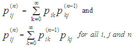 | (2) |
At this point it is very clear that the n-step transition probability can be obtained from the one step transition probabilities recursively.Suppose n = 2 then,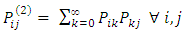 The Chapman-Kolmogorov equations implies that
  In particular,
 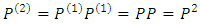 and by induction,
2.2. Theorem (Chapman-Komolgorov Equations)
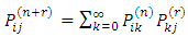 | (3) |
Think of going from  to j in n + r steps with an intermediate stop in state k after n steps; then sum over all possible k values.Proof 1: By definition,
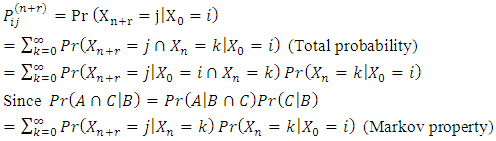 Now given a two-state Markov chain with one-step transition matrix
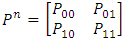
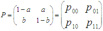 | (4) |
with 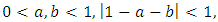 then the n-step transition matrix is given by:
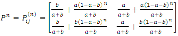 | (5) |
Proof 2: We want to show that 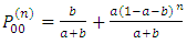
 from equation 4Proof 2: From equation 2
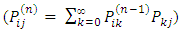
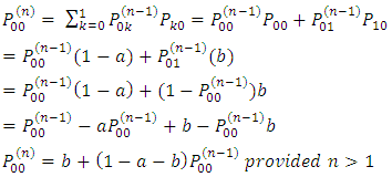 This is a recursive relation that can be used to find
  But by induction,
  (from equation 4)
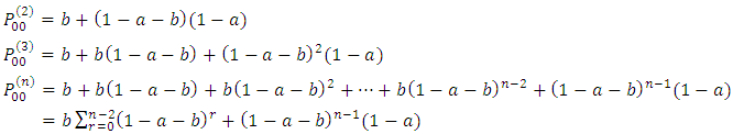 | (6) |
But 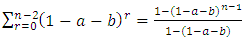 (sum of a geometric series)From equation 6,
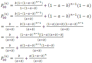 Similarly from
 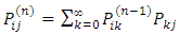 we have,
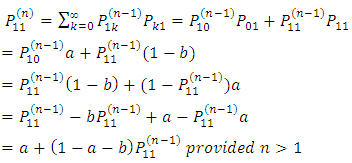 But by induction,
  (from equation 4)
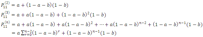 But
But 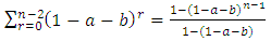 (sum of a geometric series)
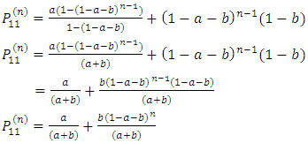 We can see that
  can be derived using the same method. However,
  can be gotten by
  respectively.
2.3. The Matrix of Flow of the Game (MF)
The matrix of flow of the game is given by: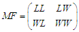 | (7) |
Where: LL = lose and lose againLW= lose and winWL= win and loseWW = win and win again
2.4. Transition Probability Matrix (TPM)
The transition probability matrix representing the game is given by: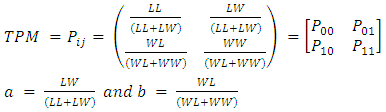 | (8) |
Probability of losing and losing again is equivalent to  the probability of winning and winning again is equivalent to
2.5. The Probability of Hitting the Jackpot (Jp)
There are a total of ninety numbers in the Golden chance lotto (That is, from 1 – 90) from which the draw is made. Five winning numbers are selected at the end of the game. For a gambler to hit the jackpot, he must get all five numbers correctly. This attracted the curiosity of estimating possible chances of hitting the jackpot. The solution to this problem lies in the possible ways in which five numbers can be selected from ninety numbers without regard to the order. One out of these selections is actually the jackpot.Thus we have: Where:
  = the total number in the pool,
 = possible winning numbers.Therefore the probability of winning the jackpot would be,
2.6. The Number of Years Taken to Hit the Jackpot 
The number of years taken to hit the jackpot if a gambler plays the game t times in a day will be: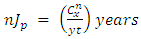 Where
Where  = total number of days in a year,
 = total number of times played in a day.
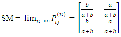
2.7. Stationary Probability Matrix for the Game (SM)
2.8. Test for Significant Difference between the Probabilities of Win, Win and Lose, Lose
The Z test for difference of two population proportions is employed since probability is proportion expressed in percentage. The Z statistic for proportion is given as: 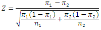 | (9) |
Where  is the average probability of lose and lose,
  is the average probability of win and win, n1 and n2 are the number of observations for population of LL and WW respectively.
2.9. Performing the Z Test
The data were fed into the R program and equation 9 was coded into the system and the Z value generated.Hypothesis 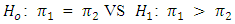 Decision RuleReject
  if
if 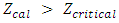 at α = 0.5 significant level, otherwise do not reject
  Conclusion If
  is rejected, the probability of losing and losing is higher than the probability of winning and winning, otherwise they are equal.
3. Results and Discussion
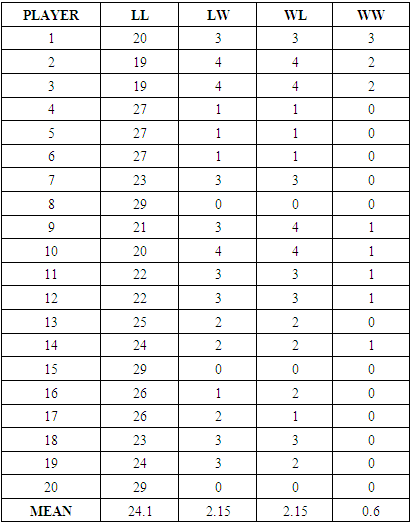
Table 2. Lottery Records
 |
| |
|
Table 2 shows the records of twenty lottery players who voluntarily entered their lottery activities for thirty days.
3.1. Results of the Analysis
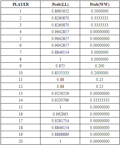
Using the R program to analyze the data, the following results we obtained:Table 3. Probability distributions for twenty players
 |
| |
|
(i) The matrix of flow of the game (MF) is generated as;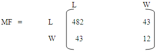 (ii) The transition probability Matrix (TPM) is generated as;
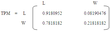 This is equivalent to a two-state Markov chain with one-step transition matrix as given in equation 4.(iii) The probability of hitting the jackpot (Jp) is generated as;Jp = 2.275351e-08(iv) The number of years taken to hit the jackpot
  nJp = 24081.79(v) Stationary probability matrix for the game (SM)
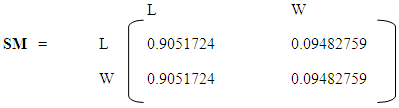
3.2. Performing the Z Test
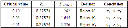
Using Equation 9, the Z test statistic  is generated from the R programHypothesis
 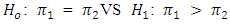 Decision RuleSince
 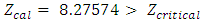 =1.645 at α = 0.05 significant levelConclusion
  is rejected, the probability of losing and losing is higher than the probability of winning and winning.
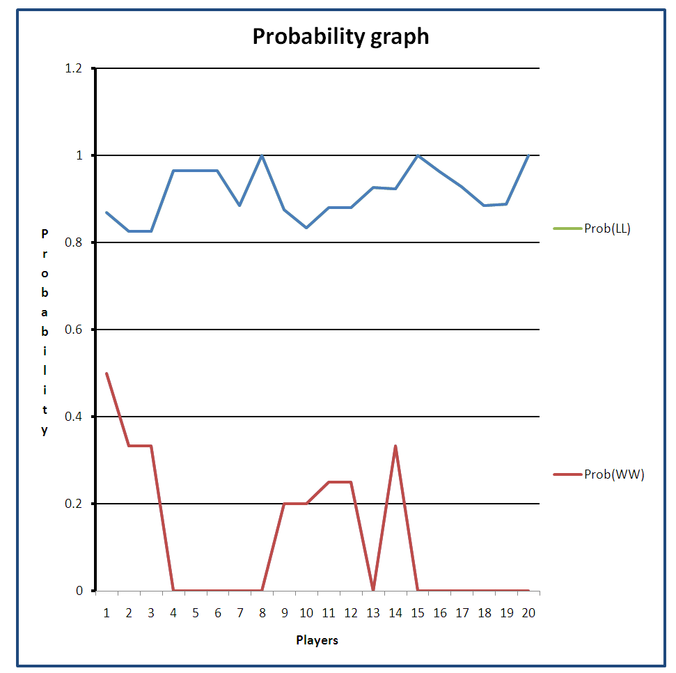 | Figure 1. Probability chart |
Table 4. Various critical values table
 |
| |
|
4. Discussion of Results
From the analysis carried out on the lottery records gathered so far using the R program, the following were observed:(i) The probabilities generated from the lotto records revealed that the chance that a lottery player would win and win again is 0.21818182 whereas the probability that the same player would lose and lose again is 0.9180952. This explains the reason for the high losses incurred by lottery players no matter how hard they try.(ii) The probability that a player will hit the jackpot (Jp) is 2.275351x10⁻⁸. This is equivalent to one out of approximately forty four million. When this digit is placed on a 4 to 7 decimal point system it will return zero.(iii) If a player plays a lottery (Golden Chance Lotto) five times daily, it will take approximately twenty four thousand (24081.79) years to hit the jackpot. An almost impossible situation.(iv) As the number of times one plays the game increases, the probability of winning and re-winning tends to be constant at 0.09482759. Consequently, the probability of losing and re-losing tends to be constant at 0.9051724.(v) The chances that one will lose and lose again are far higher than the chances that one will win and win again.(vi) From the probability graph, it is observed that the probability that a player would lose and continue to lose is between 0.8260870 and 1; whereas the probability that a player would win and continue to win is between 0.0 and 0.5.
4.1. Conclusions
It is clearly observed from this study that lotteries have an extremely low probability of winning. The 5/90 lotto carries a one in 44 million probability of winning. Thus if all the possible numbers are listed out, the only way one could be sure of having a win is to get as many as 44 million people who will each play one of the number combinations. In this case one person wins the jackpot but 43999999 persons lose. Definitely, this is not a wise venture. With an extremely low probability of winning and the very low payout ratio, buying lotteries is evidently a losing proposition. Obviously, the house always wins why the gambler loses at all times as the payout money at any point is part of the losses of other gamblers.
References
| [1] | Ashong A., (2020): A Lotto Operator was fined by the National Lottery Regulatory Commission for failing to pay its winners. Retrieved from: www.ghgossip.com. |
| [2] | Barnes G. M., John W. Welte, Marie-Cecile O. Tidwell, and Joseph H. Hoffman. (2011) Gambling on the Lottery: Sociodemographic Correlates Across the Lifespan. J Gambl Stud 27(4): 575–586. https://doi:org/10.1007/s10899-010-9228-7. |
| [3] | Beckert J. and Lutter M. (2008) The Inequality of Fair Play: Lottery Gambling and Social Stratification in Germany. European Sociological Review, Volume 25, Issue 4, 475–488, https://doi.org/10.1093/esr/jcn063. |
| [4] | Burger A.P., Grundlingh W. R. and Jan H van Vuuren (2003). The Lottery Problem. Retrieved from: https://www.researchgate.net/publication/228998461. |
| [5] | Clotfelter, C.T. and Cook, P.J. (1989) Selling Hope: State Lotteries in America. Harvard University Press, Cambridge MA and London. |
| [6] | Clotfelter, C.T. and Cook, P.J. (1991) Lotteries in the real world. Journal of Risk and Uncertainty 4, 227–232. https://doi.org/10.1007/BF00114154. |
| [7] | Doll Jen (2012). A Treasury of Terribly Sad Stories of Lotto Winners. The Wire Retrieved from www.theatlantic.com. |
| [8] | Grote, Kent R. and Matheson, Victor A. (2006). In Search of a Fair Bet in the Lottery. Eastern Economic Journal 32 (4): 673-684. |
| [9] | Keen Brittany, Anjoul Fadi And Blaszczynski Alex (2019) How learning misconceptions can improve outcomes and youth engagement with gambling education programs Journal of Behavioral Addictions 8(3), pp. 372–383. DOI: 10.1556/2006.8.2019.56. |
| [10] | Kucharski, Adam (2016) The Perfect Bet: How Science and Math Are Taking the Luck out of Gambling NEW YORK: BASIC BOOKS ISBN 978-0-46505595-1 Retrieved from https://doi.org/10.1007/s00283-019-09925-4. |

 Abstract
 Reference
 Full-Text PDF
 Full-text HTML