1. Introduction

Forecasting production and its consumption electric elements are a major area that utilizes different models and future forecasting. Different models are used for getting prediction about the pattern of future behavior. A satisfactory degree of statistical validity obtains through every energy series according to optimum forecasting models. And also establish regional energetic planning according to their requirement. There are two main models utilize in the forecasting production and consumption electric according to nature of requirement. These models involve Fuzzy time series and Fuzzy C-Means. Fizzy time series and Fuzzy C means have their abilities and according to their nature of performance, they both handle a different kind of data according to their utilization [1].

The concept of the fuzzy group and the fuzzy logic, which was proposed by the Azerbaijani scientist of origin, Lotfi Zadeh in 1965, was subsequently applied in a wide and varied manner to different systems, especially the complex Ones, as the increase in complexity in the systems increases the uncertainty and thus leads to a lack of information and the term uncertainty emerged, To reinforce the position of probability theory.

The theory of probability and the theory of fuzzy groups facilitate two types of uncertainty, which generally come as a result of two reasons, the first of which is the method of measurement to reach new knowledge and the second is the natural language for communicating with others in order to deal with the problems of uncertainty. The probability theory can be successfully applied to large areas of science because it is concerned with treating the occurrence of Random future incidents based on currently available information. Despite the success of probability theory, it is still unable to show uncertainty with high accuracy, and it is also unable to show uncertainty in the results either. Controlling the linguistic terms expressing natural characteristics such as length, temperature, etc. have contributed to the emergence and development of the Concept of the fuzzy group.

Cluster analysis is one of the methods used statistically to classify data primarily into a set of nodes (clusters). Each cluster contains a set of data that have common structural characteristics and this is preferred by most methods of distinguishing patterns because the data will be distributed over a number of clusters so that each cluster contains Elements have similar characteristics among themselves, which requires that there be separate clusters from each other, so that each pattern belongs to one cluster and only one in the case that the clusters represent regular groups. As for the fact that the clusters may represent fuzzy groups, the cloudy cluster makes the concept of fragmentation wider in a way that allows any pattern to have a relationship of belonging to any of the clusters using a membership function that ranges between zero and one so that the value of the membership function of any type indicates higher Reliability for belonging of this pattern to a particular cluster. The output of the fuzzy cluster algorithms is called fuzzy segmentation. These algorithms and methods occupy a wide area in research and studies and in all fields. The most famous techniques of the fuzzy cluster are the fuzzy-c-medium algorithm or method, abbreviated as FCM, which was proposed by Besdek more than 25 years ago. As for the fuzzy time series, it was proposed in 1993 by the two scientists chissom and song and they developed two definitions of the fuzzy time series models that are not time variable and time variable and which are used in the forecasting. The time series is defined in terms of relationships, and the final step involves raising the fuzziness defuzzification of the predictive results. Most Studies and research in the field of fuzzy time series are concerned with the methods of forming the fuzzy group and the fuzzy relationships. There are fuzzy time series from the first order and higher ranks depending on the logical relationships between the fuzzy groups and research trends in this field include methods of forming fuzzy groups, the most famous of which is the method and research directions are divided into Several trends regarding the effect of the number of fuzzy groups, the order of the fuzzy time series, and the defuzzification methods on the accuracy of the prognostic results.

2. Summary of Literature Review

Fizzy Time Series is an algorithm, which, is used in the processing of huge data. It is a model used for programming for data processing in different languages including Java, Ruby, Python, and C++ as well. By using multiple machines in the cluster, large-Scale data can be analyzed by using parallel nature Map Reduce programs in nature. There are four stages from passing these, Map Reduce can only work properly and can provide efficient and excellent results successfully. These four phases are mapping, splitting, reducing and shuffling [2].

A chunk of input that by the consumption through a single map is divided into fixed-size pieces to process is efficiently and hence these Input slits make the processing quick and easy. In the time series program, the first step is the Mapping. To produce output values, the data from each slip to a mapping function passed in this phase [3].

The mapping phase output is consuming in this phase as it is going to consolidate the output from the mapping phase into relevant records. Along with their respective frequency, the same words are clubby together. The output values are aggregate from the shuffling phase. A single output value comes in return for this phase after shuffling [4]. The complete data set is summarizing in this phase [5].

Usually at the reliability level of data Centre and usually at scale Cloud computing is designed to provide on-demand resources and services to programs on the internet. Along with Map Reduce cloud computing works and this increases the efficiency of working of both the programs in programming or processing of data [6] [7]. As discussed above, Map Reduce helps to process data through its programming model that is specially designed to process a large amount of data efficiently after dividing that large amount into small chunks. There are some capacity-on-demand styles of clouds that support the parallel programming of Map Reduce which are Google's Big Table, Hadoop and sector [8].

Accuracy in the forecasted value is the major problem in the fuzzy time series forecasting. New techniques for fuzzy time series forecasting also introduce that used different parameters to generate better results. For forecasting, a different approach also utilizes that is known as a simplified computational approach according to proposed methods [9].

In a particular domain, the time series is an orderly sequence of values of different variables. In the area of time series analysis, challenging tasks are part of forecasting techniques.

In the area of tourism, agriculture, employment, climatology and economy forecasting show significant impact on the decision making area. From natural calamities, timely forecast help to save from any loss. As an emergent research area, fuzzy tie series forecasting is acted in this regard. It handles a different kind of problems according to imprecision, vagueness ad uncertainty [10].

Forecasting methods and time series analysis are very commonly used in different areas like meteorology, economy, medicine and engineering according to the nature of work [11]. From the traditional and consecrated statistical tools to the new computational intelligence tools according to several methods of analysis and forecasting, fuzzy time series is most effective methods and it provides many attractive features to its users like scalability, simplicity, manageability and readability [12].

The asset is defining as a dichotomy where every element involves in the set according to logical theory and classical mathematics. It imposes inflexible and strong boundaries according to a valuable set of data. Because innumerable realities are not so effective for the human being so this dichotomous way of thinking is not convenient. The logic of Fuzzy imposes the duality instead of dichotomy that may belong to different set to a certain level and sometimes belong with each other with the strong member’s ship of each value [13], [14].

Time series is a combination of different data according to the behavior of random variable overtime and their analysis must take into account the order in that were collected and successive record of this variable are not independent of each other. According to Ehlers, it is interested in analyzing and modeling this dependence and the neighboring observation are dependent, which show that past or lagged value of the same series are used for predicting future values of time series. Autoregressive model is considered a simple example where P show lagged variable utilize in the forecasting model [15].

The idea of time series s divides into fuzzy sets and study in-depth about behaves in every area. As value jump one place to another, how the partitions related to themself over time according to rules of this model. The fuzzy time series methodology can be distributed into two procedures one is training and the next one is forecasting [16], [17].

Training procedures involve some basic steps to consider the utilization of this procedure according to fuzzy time series which include Definition of the Universe of Discourse U, create the Linguistic Variable A, Fuzzyfication, creating the temporal pattern, creating rules and with these steps, there are also many benefits of this procedure like it is easy to update and attractive for mostly changing data and it is easy to parallelize that has also become attractive for the major data [18].

Forecasting procedures help to determine the future data according to prediction and utilize this procedure after proper training to handle the data. This procedure involves many steps like input value fizzy fiction; find the compatible rules and De-fuzzy fiction [19]. These two procedures help the fuzzy time series forecasting according to data and its nature of utilization [20].

It is also a contested concept because of 'ambiguity' over the concept and definition of security. Every other scholar has defined security following what they feel the security to be. Some various factors and variables are needed to be addressed if we aim at achieving 'maximum security' in a state [21].

Also, we have to define and realize what security is for. At what risk and at what cost we are seeking. What can be the possible road map to achieving security? As stated above security is a contested concept with everyone having their version of security? A complete algorithm is developing by using the historical data and utilizes them for forecasting process according to this proposed model [22].

Now with the fuzzy time series forecasting model, we are also discussing the Fuzzy C-Means model for the forecasting production and consumption of electricity. Fuzzy C-Means algorithm is utilizing the incorporated spatial information for clustering according to member functions. For economic prosperity, there should be a well-planned and efficient transport network because they can affect the society and natural environment and could play an important role in transforming communities with proper planning and strategy. Safety is a critical aspect of the Electric consumption system and it must be catering while planning and strategizing Electric consumption system. Safety is not limited to any person or living thing, it caters the environmental safety, land safety and safety for the societies [23], [24], [25].

To tackle the Electric consumption issues or planning for new Electric consumption facilities than it should contain

A feasibility report, of whether it will be facilitating the economy or not. The feasibility report tells us how long this system or policy can go and what benefits could be taken. There should be enough planning of moving long vehicles with short vehicles and plans to tackle traffic jams in rush hours. This is an important part of planning to keep in mind about the movement of goods containing vehicles. Planning of Electric consumption and land goes side by side to accommodate the effects of land use on Electric consumption demand and supply and the effects of Electric consumption on land. There must be provided ways through which achievement of social goals will be attainable through Electric consumption systems. Identification of those strategies is important which provides access to persons with disabilities and improves public health and safety with the help of improving air quality and reducing road collision [26].

This research is written by Mahadevan, Sharma and Banerjee in which they have discussed the energy importance within the framework of network devices. For the enterprises and data Centre networks, energy efficiency is becoming increasingly important for operating networking infrastructure. The researchers have proposed many strategies to manage the power consumption of network devices. The strategies emphasize on the usage of a variety of switches and routers which will be useful to save the power of various network devices [27] [28]. In this paper, authors have discussed the hurdles in network power instrumentation but they have also provided the study of power measurements such as varieties of networking gears which includes wireless access points, routers, core switches, and edge switches [29].

They have built a benchmark through which users will be able to measure the power consumed by each device and also could be able to compare the power of each device [30]. In today's world, energy efficiency is the main point or agenda of every company and firm without which the company could not be able to reduce their costs. Now a day's only energy-efficient companies should survive for years. A study shows that the US is consuming 6.06 Terra Watt Hours through networking devices yearly [18].

In the case of large data, VL data options are used according to large data requirement in the management of data sets. In different applications, data mining communities to search VL databases and clustering is one of the basic tasks used in pattern making and its recognition. Algorithm of clustering is considering very important to well scale the very large data and effectively used in many dimensions. To extend fuzzy C-Means clustering to very large data, three different efficacies according to implementation techniques are used according to the need of data [31]. Next, the incremental techniques that make one sequential pass through subsets of the data and the last one are sampling followed by no iterative extensions [32].

In the end, they make experiments which include shutdown overhead and energy consumption. They stated that power management is the mainstream of embedded systems and lays down different important aspects for these systems. The power management can lead the embedded systems to longer battery life as well as it will provide static power consumption. The consumption of power is reduced due to the switching of energy [33]. They said that the development of dynamic voltage scaling is designed to minimize dynamic power consumption which is a dominant factor. Due to the time and energy cost associated with shutdown, longer shutdown intervals are better [34].

When clustering the unlabeled data, fuzzy possibilities C-Means and algorithm also generate membership and typically values. The sum over all data points of typicality to a cluster is one when the FPCM constrains the typicality values according to requirements. For large data sets, the row sum constraints produce unrealistic typicality values as par nature of the information. a new kind of model utilizes in this regard which is known as possibility fuzzy C-Mean model. With the usual point prototype or cluster centers of each cluster, PFCM produces membership and possibilities al the same time according to the requirement of data [35].

They have discussed the importance of power, and what are the characteristics of the power model. They also critically examine the speed of power and make real-time scheduling. Their real-time scheduling includes DVS and critical speed, shutdown overhead, and computation has been done through algorithms. The concept of security has long been a neglected and limited concept for the world [36] [37]. In reality, the security is vast and a very important concept that is for the reason that countries take extreme measures over the context of security itself. As stated above security in past was only associated with the use of hard military power but in contemporary times, the concept of security has changed [38].

The different comparison also presents between FCM and PCM with the PFCM according to different data sets. It also explains that both types of comparisons are favorable for the models and generates better outcomes. The following piece of writing is an attempt to re-define the core concept of security. Every time the word 'security' comes up, it is treated or is usually associated with 'Hard military power'. While there are many with various proposals considering issues like poverty, drug trafficking.

Economic is part of security. It is very important to identify various aspects of security because with time the concept of security changes [39].

3. Basic Concepts Fuzzy Sets and Their Properties & Crisp Set

3.1. Set Crisp

A set crisp is defined as a collection of elements and objects That is the element x belongs or does not belong to the group A and , Where is the overall group and when it is said that this statement is either true or false and that all elements of the universal group U can be determined to be either members or not members of group A, which we can know Function characteristic [40].

This function of group A is symbolized by the symbol , and its formula is as follows:

(3.1)

To overcome the limitations of the traditional (classical) group theory in its definition, the idea of fuzzy groups was defined as an expansion of the traditional groups as it has imprecise (blunt) boundaries.

3.2. Fuzzy Set

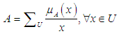
Let group A be within the universal group U, since each element in U can be an element in A, but the degree of its membership is determined by a real value within the period [0,1] and that the membership function of group A is defined as follows:

There are an unlimited number of organic functions, the most famous of which are the trigonometric, trapezoid, and bell-shaped function. Through this expression, it is possible to obtain complete information about the degree of membership of any element in A within the universal group U if represents the degree of membership for element x within the group A and the fuzzy group A is expressed by ordered pairs for each element and its membership function, as follows:

(3.2)

There are other expressions for the fuzzy group A, so if the universal set U is discrete, the fuzzy group is written as:

(3.3)

3.3. Linguistic Variables

Fuzzy numbers are often used to represent quantitative variables, and they are called these

Numbers in the name of linguistic variables, linguistic variables are an expression of words or sentences in the form of numerical values, all values taken from a group of expressions (terms) that contain a set of acceptable values and its elements are in the form (value / concept). And each (value / concept) in the expression group is expressed in a fuzzy number and is known to the global period or part of it is called the base variable, and in short, this relationship is expressed as

3.4 Fuzzification

It is the process of converting assertive fragile values into fuzzy ones, using the organic functions of fragile values that take different shapes, including trigonometric, semi-trapezoid, and natural... etc. and whose membership values are limited between zero and one. There are different ways to do this that can be carried out through intuition, genetic algorithms, or neural networks.

3.5. Defuzzification

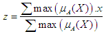
It is the process of converting fuzzy outputs into fuzzy outputs that take real numerical values and this is done in several different ways and is done in several ways by raising the Defuzzification, including:

a. Max-membership principle

In this rule, the value of Z after raising the Defuzzification is equal to the value of x with the highest organic degree, expressed as:

(3.4)

Since is the value that has the highest degree of membership in the fuzzfied group A, and if we take the following example for group A = 0.3 / 10 + 0.45 / 12 + 0.6 / 15 + 0.9 / 17 then Z = Max (A) = 17.

b. Centroid Method

This method is widely used, and it is also called the center of gravity method or the area center method, and in the case of the membership function it is known as discrete

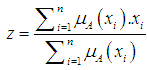(3.5)

c. Weighted average method

This method is only applicable to symmetric membership functions, and it bears some resemblance to the centroid method except that it takes maximum degrees of membership functions only and its formula is as:

(3.6)

3.6. Some Definition Related To Fuzzy Time Series

Fuzzy time series was first defined by the two scientists Song and Chissom in the year 1993, and the concept of fuzzy time series can be described in the following terms:

Suppose U is a crowd of things representing the universal space ending where the fuzzy group can be defined with respect to U by the equation

(3.7)

Where a membership function is fuzzy set so

(3.8)

If the membership is from is the degree that is owned by against .

3.6.1. First Definition: Fuzzy Time Series

Let Y (t) (t =..., 0,1,2,...) subset , become a universe discourse with the fuzzy set defined and F (t) is a collection of then F (t) is called fuzzy time series defined in Y (t) (t =..., 0,1,2,...). From this definition F (t) can be understood as a linguistic variable of the linguistic probability value F (t) [41]. Because at different times, the value of F (t) can be different, F (t) as a fuzzy set is a function.

From time t and universe discourse is different at each time so Y (t) is used for time t (Song and Chissom, 1993).

3.6.2. Second Definition: Fuzzy Relationship

Suppose F (t) is caused only by F (t-1) and appointed with then there is Fuzzy Relations between F(t) and F(t-1) expressed by the formula

Where is the Max-Min composition operator. The relation R is called the first order model F (t).

Furthermore, if the fuzzy relation t is time independent so for different times

So that F (t) called time-invariant fuzzy time series.

3.6.3. Third Definition: Invariant Fuzzy Time Series Time

Suppose F (t) is caused only by F(t-1) and appointed with then there is Fuzzy Relations between F(t) and F(t-1) expressed by the formula

(3.9)

Where "R" is the Max-Min composition operator. The relation R is called the first order model F (t).

Furthermore if the fuzzy relation R (t, t-1) of F (t).

t is time independent.

And if

So for different times so that F (t) called time-invariant fuzzy time series and the opposite of this called time-variant fuzzy time series [42].

3.6.4. Fourth Definition: N-Order Fuzzy Relation

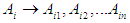
If F (t) is produced by several fuzzy sets

F (t – n), F (t - n +1)... F (t -1)

Then the fuzzy relationship is symbolized by:

Where

And such relationships are called order fuzzy time series.

The concept of the nth time series was proposed by Chen in 2002 and used to predict the number of students admitted to the University of Alabama.

3.6.5. Fifth Definition: Fuzzy Logic Relationship Group

Relationships on the same fuzzy group on the left end can be grouped into a group of relationships, let's assume that they are fuzzy logical relationships in the form [42]:

(3.10)

It can be grouped into a group of relationships as follows,

And no fuzzy group can appear at the right end more than once. The term relationship group first appeared from scientist Chen in 1996.

4. Methods

4.1. Chen Method Review

This method is a simple model proposal that includes simple mathematical operations. The suggested step-by-step procedure can be described as the following steps:

1- Dividing the discourse of Universe into periods of equal length

2- Defining the fuzzy groups on the global event.

3- Fuzzify historical data.

4- Identify fuzzy relationships.

5- Establish groups or groups of fuzzy relationships.

6- Defuzzify the forecasted output.

The steps involved in the Chen method

Step one: The first step: Define the global event and divide it into periods of equal length. The global event U is defined

Where and are the corresponding positive numbers, they are chosen to complement the minimum and maximum values to be indivisible values, which facilitate their calculation.

Where and , they are the lowest and highest data values, respectively. The global event is divided into several periods. For example, if the number of periods is 7,

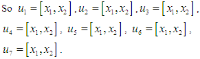The second step: Defining the fuzzy groups on the global event. Suppose that is the fuzzy groups as they are linguistic values of the linguistic variables of the data under study. Fuzzy groups identify the global event as

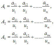Whereas and and

And represents the degree of membership for the assertive period in the fuzzy group.

Before defining the fuzzy groups as U, the syntactic values must be assigned to each fuzzy group.

Fuzzy groups can define a wild event as follows:

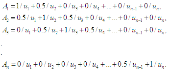In general, the expression can be written as [43]

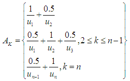(4.1)

The third step:

Fuzzy data historically in this step the fuzzing process is to distinguish sums between the historical values in the data sets and the fuzzy groups defined in the previous step; each historical value is fanned according to the highest organic score. If the highest degree of affiliation is certainly as a time variable, say F (t-1), it appears in the fuzzy set , then F (t-1) Fuzzify the set . Let us take the example that we wanted to fluctuate the value at the year (1970), so we calculate the highest degree of belonging to the value in any period, let it be , so F (1970) is in group , but the value at year (1971) has the highest degree of affiliation in the period , so F (1971) fog to set and so on for all data.

Step 4: Distinguish Fuzzy Relationships In this step; relationships are distinguished from fuzzing historical data. If the time series variable F (t-1) is fuzzed in the fuzzy set and F (t) in then is related to . 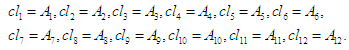And we symbolize this relationship in the form , where in the current case and is the subsequent case of the statement value for a particular year, and from the example in the previous step we can say that the relationship between (1970) and (1971) is and is called the left hand side, and right hand side, and so on for all data, Note that it is not possible for repeated relationships of the same type only once and ignore the rest.

The fifth step: This step can be summarized as establishing fuzzy relationship groups. If the fuzzy group has a fuzzy relationship with more than one group, then the groups on the right side are merged or grouped more than once. This is called establishing fuzzy relationship groups. As an illustrative example, the establishment of relationship groups is in our paper Scientific is as

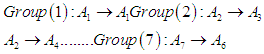Step 6: Raise the fuzziness to calculate the predictive results and assuming that the fuzziness is for the value of the indication from F (t-1) it is The results of the prediction of F (t) are determined according to the following principles:

1- If there is a one-to-one relationship (1-1) in the relations group for , say , and the highest degree of affiliation with is in the period , then the results of the prediction for F (t) are equal to the midpoint of the period.

2- If is not related to any other group, i.e. where is the empty group, and the highest degree of affiliation with is in the period , then the results of the prediction are equal to the middle of the period .

If there are one-to-many relationships in groups of fuzzy relationships of , let's say , and that the highest degree of affiliation occurs in interval , The results of the forecast are calculated by finding the average midpoint for the periods and by formula this model that has been presented is called a fuzzy time series model of the first order, and Chen has provided models The steps for finding a prognosis are the same as the previous method with a difference in the formation of the fuzzy relationships.

4.2. Fuzzy C-means Method Review

The FCM method is also called Fuzzy ISODATA, which was proposed by Bezdek in 1981 [44], [45].

The algorithm for this method represents a clustering technique separated from Hard c-means (HCM), so the HCM algorithm is based mainly on the philosophy of Crisp Set, which uses the strong hard partitioning of data points, so that the deterministic determination of the affiliation of these points: whether it belongs For a specific cluster or not, as for the FCM algorithm, it is based on the philosophy of fuzzy logic, which mainly depends on the idea of gradual belonging and fuzzy partitioning, which allows each data point to belong to a cluster with a specific degree to an organic degree, and thus each data point can belong to several clusters in the n One with different degrees of membership falls in the period [0,1].

If we assume that the data set is a finite subset of the set of real numbers. Let us assume that c is the number of clusters and it is an integer such that, so the FCM algorithm splits the data set X into c from fuzzy clusters, so that the data in the same set are as similar as possible and differ from other different groups as much as possible.

Thus, the fuzzy hash of the datasets X can be represented by the membership matrix U with dimensions so each entry in the U matrix is denoted by and is within the range [0,1].

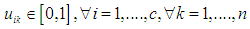(4.2)

The goal of the FCM method is similar to what is found in the HCM method, which is to find the center of each cluster and reduce the objective function according to specific constraints, which can be represented by the following equation:

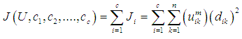Where is the target function within the cluster i is the Euclidean distance between the data point and the center , and the J function is reduced according to the following restrictions [46]:

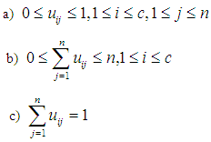(4.3)

Each element may belong to several clusters of varying degrees of membership, but the conditions (a) and (c) require that the final sum of the values of the membership functions of any element be equal to one[47], [48], [49].

As for , it represents the degree of membership of the data point to the center of the cluster and is within the range [0, 1] and that the parameter M: is Membership Weighting Exponent, , In order to achieve a reduction of the objective function, there are two conditions represented by the two equations as follows:

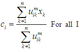(4.4)

Whereas the center of the cluster i and i = 1, 2, 3…c

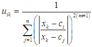(4.5)

To find the predicted values using this method, we will use the FCM algorithm, as the data is entered in the form of vectors, the number of clusters c is selected, specifically the threshold value, and the value of m is determined. And then using the outputs of this algorithm which are clusters of c number which includes the elements after being classified, the number of iterations, the membership matrix U, the centers matrix, and the objective function.

The steps involved in the Chen method

The first step: Defining the comprehensive group U that contains all the study data, where

The second step: Divide the comprehensive set of several clusters using the FCM algorithm, which will produce clusters containing a set of data that are similar to each other

The third step: Defining the fuzzy groups on the global set suppose that is the fuzzy groups, so they can be defined in the form:

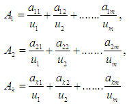Whereas and and

And represents the degree of membership for the assertive period in the it is a component of the membership matrix U.

Fourth step: fuzzfied the data. This step is done by testing each cluster in the form of a fuzzy group. Each value entered represents the highest degree of affiliation within a given cluster, which appears in the membership matrix that was mentioned previously, is fuzzfied to the fuzzy group equal to that cluster. Let us say that the entered value of for the year 1970 falls within the first cluster, then (1970). Thus for all the entries, the historical data are fuzzfied according to his fuzzy group.

As for the remaining steps (from the fifth step to the last they are similar to the previously mentioned steps within the Chen method and for the first and second order.

4.3. Suggested Method for Predicting Using FCM Review

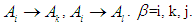
Through our study of the fuzzy meshing methods such as Chen method and the fuzzy C-medium FCM method, and we obtained the results of prediction for it, and in order to develop the previous methods to obtain better results for the values of the prognosis according to the ideas studied in this research, we proposed a method that includes the same previous steps except for the step for reconstructing the fuzzy relations groups and is as follows : Reconstructing the fuzzy relationships of the group of fuzzy groups is the most important step in this method, as the relationships between the group of fuzzy groups are raised (trimming) the relationships between the group of fuzzy groups are rebuilt according to special rules, meaning that if and the predictive value of the group of uncertain depends on the group then Relationships group promises to be formed by the proposed relationship

So we had the relationships

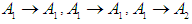
Therefore, the results of the prediction will be close to the real results. If we take the example the new relationships will be according to our proposal in the form

Then

This method is somewhat similar to the median method as one of the measures of central tendency in statistics.

5. Application Phase, Results and Discussion

5.1. Introduction

This section includes three applications of Chen method and Fuzzy Time Series c-means and Suggested Method on data representing the amount of production and consumption electric for the years (2015_2016). The first application deals with the Chen method, the second application of the cluster method is the fuzzy c-medium method FCM, and finally a Suggested method for forecasting using FCM. Using different organic functions to find the organic values of the elements in the fuzzy groups, and also using the fuzzy relationships of the first and second order, and the extent of the influence of all these elements on the results of the prediction was clarified.

The ready-made program (MATLAB 2012), excel was used to divide the data into the required clusters by FCM method, and also to find and plot the values of membership scores and plot fuzzy time series.

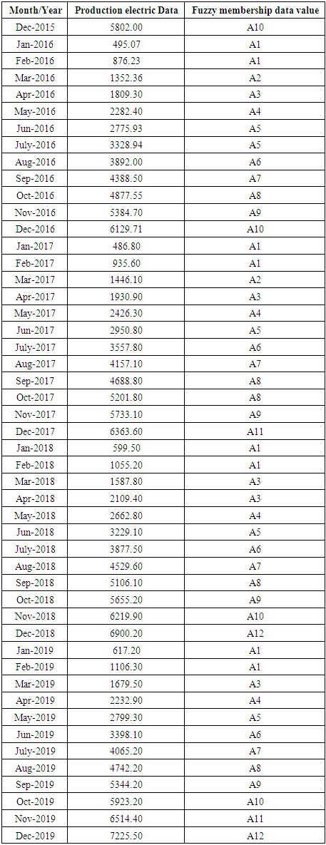
5.2. Data Description

The data used in the application represent the amount of production and consumption electric in china for the years (Jan 2015_Dec 2019) and its range ranges between (400_6900) GWh. From observing the data, we find that it is characterized by instability and varies from month to month randomly. We have dealt with this data because of the importance and great impact of production and consumption electric. On our daily life and its impact on the economy, agriculture, etc. as well as floods, Figure (1) and figure (2) represents a chart of the time series of production electric and consumption for each month.

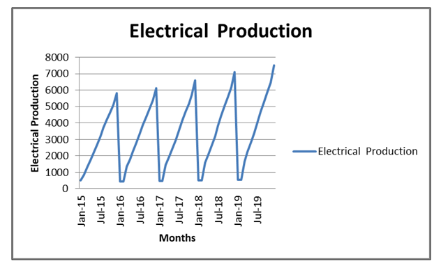Figure 1. Production electric Time series of the amount of electricity production from the time period (2015-2019)

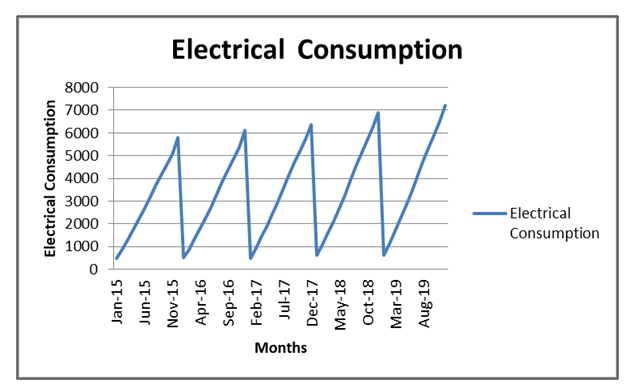Figure 2. Consumption electric Time series of the amount of electricity consumption from the time period (2015-2019)

5.3. Model Evaluation

The process of evaluating models is intended to evaluate the field suitability of the model for the pattern in which the series data is running or the accuracy of the model in predicting the values of the current and future series, and there are many measures of the suitability of the model all depend on the degree of error, which is the difference between the actual value of the series at a specific time And the string value that the model expected at that time. In this study, we will rely on the following methods to compare the two models used in this paper to find out which one is more accurate in prediction.

5.3.1. Mean Absolute Percentage Error (MAPE)

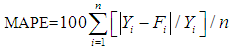(5.1)

The mean absolute percentage error (MAPE), is a measure of prediction accuracy of a forecasting method in statistics, for example in trend estimation, also used as a Loss function for regression problems in Machine Learning. The MAPE (Mean Absolute Percent Error) measures the size of the error in percentage terms. It is calculated as the average of the unsigned percentage error.

5.3.2. Mean Absolute Deviation (MAD)

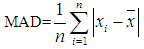(5.2)

The median absolute deviation is a measure of statistical dispersion. Moreover, the MAD is a robust statistic, being more resilient to outliers in a data set than the standard deviation. In the standard deviation, the distances from the mean are squared, so large deviations are weighted more heavily, and thus outliers can heavily influence it.

5.4. Result Chen Method and Discussion

In this method, we will find forecast values for the state of electricity production in the period between December 2015 and December 2019.

The universal set U must be divided into several equal intervals. In our case, this set U is divided into twelve intervals equally.

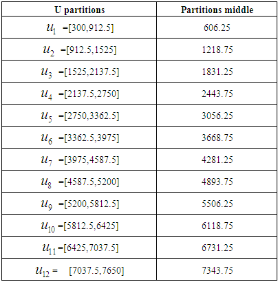
The first Step; define the global event where is the smallest value (Jan 2019), is the greatest value (Dec- 2019), Thus, the universal set U will be as follows: U= {300, 7650}.

And then divide U into equal intervals in length, which is in the table 5.4.1 below:

Table 5.4.1. Dividing periods

The second step is to define the fuzzy groups on the global event, so the fuzzy groups are

As linguistic expressions in the form

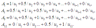And the value of the organic function for the fuzzy groups is calculated as

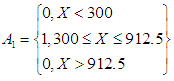And so on for the rest of the groups.

The third step, which is fuzzification the historical data, was on the basis of the highest degree of membership within the periods. Let us take the first value, because it has the highest degree of affiliation in the period , so (1970) F is in the group and the second value is, it has the highest degree of affiliation in the period also, so (1971) F is fuzzifed In the group, and so on for the rest of the historical values, as shown in Table 5.4.2 below.

Table 5.4.2. Fuzzification historical data

The fourth step is identifying fuzzy relationships. From the definition of fuzzy relationships, you find that the time series variable F(Apr-2016) is fuzzfied into and F(May-2016) is fuzzfied into , so relates to and we denote it by the symbol , and F(May-2016) is fuzzfied into so relates to so it is denoted by .

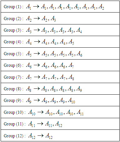
The fifth step represents the establishment of groups of fuzzy relationships. From Table 5.4.3, we notice that the fuzzy groups have a fuzzy relationship with more than one group, so the groups are merged or grouped on the right side, noting that no fuzzy group is repeated on the right side, so we notice that the group It has a relationship.

With and becomes the first group in the form: Group (1):

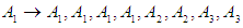The following table 5.4.3 shows groups of fuzzy relationships

Table 5.4.3. Fuzzy Relation Group sets

The sixth and final step is to raise the fuzziness to find the results of the forecast, and this step depends on the previous step.

From the first group ,

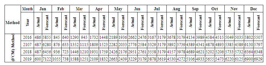
In this group we can find the value by Partitions middle.

Contains mid intervals of U partitions table 5.4.1.

Forecasting value Example: 5814, 57*1/2 "of A1"+1875*1/2 "of A2"+ 2925*0 "of A3"+...+ 7125*0 "of A12"=5320.3125. This forecasted value looks much greater than the real value in Jan-2016 = 453, 09. That’s means we will see high MAPE and MAD. We will see the next method in the next section.

Table 5.4.4 and Table 5.4.5 below show the actual and forecasted values of production and consumption electric for period from January 2016 to December 2019 in GWh the result has been rounded to the nearest integer.

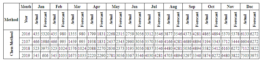Table 5.4.4. Actual and forecasted values of production electric in GWh

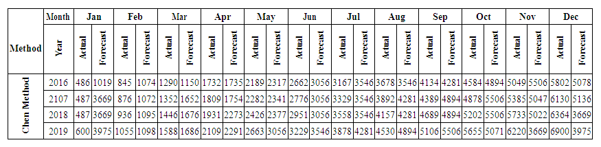Table 5.4.5. Actual and forecasted values of consumption electric in GWh

5.5. Result Fuzzy c-mean (FCM) Method and Discussion

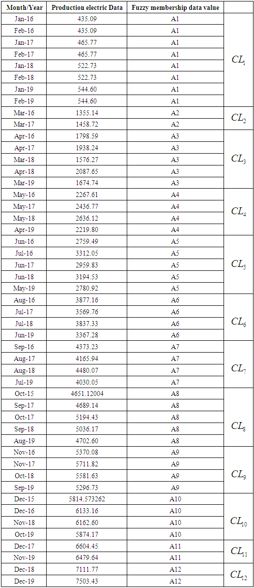
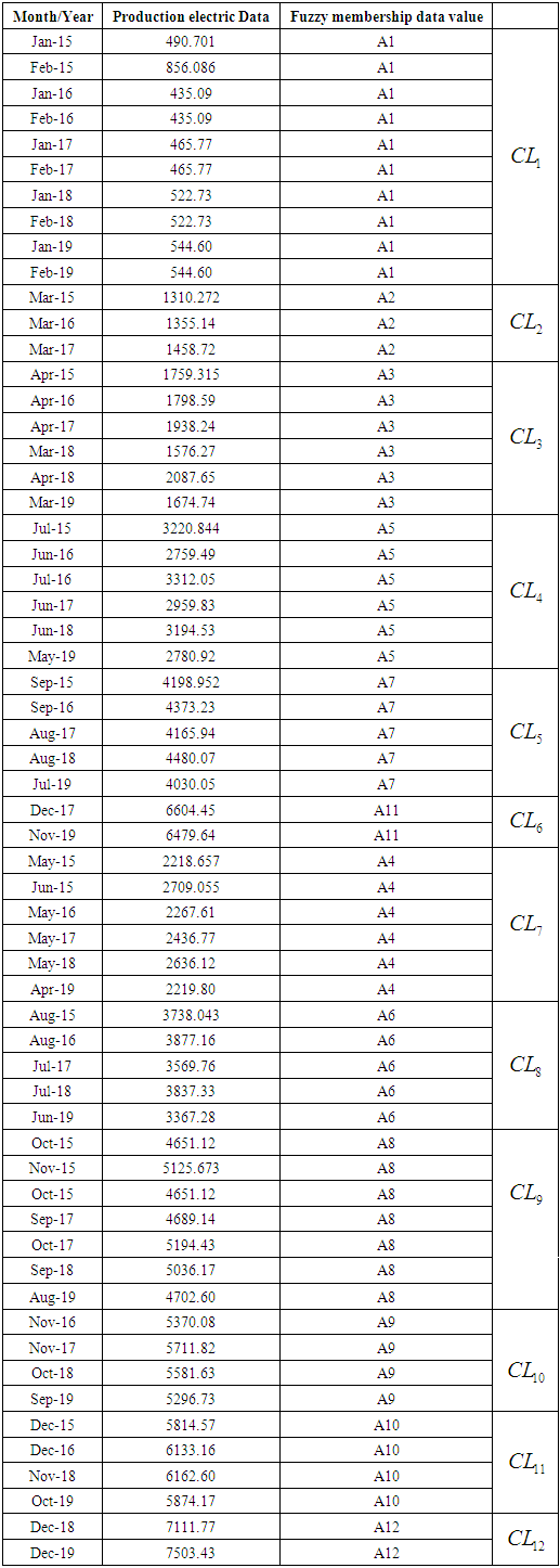
In this model we will present the application in finding the predicted values of the data shown, and as we mentioned in section 5.4 the method of finding the clusters that we will use in finding the values of the prognosis and the number of clusters (5_12) clusters and by using the Gaussian natural membership function for the first order.

The first step is to define the data set. The second step is to determine the number of clusters and find the group of each cluster. We have dealt with the number of clusters (12). As for the rest of the results, we will mention them in an appendix of the results. And using MATLAB or excel program, the ten clusters and its contents were determined from the data used, and the results were as shown in Table 5.5.1 below:

Table 5.5.1. Clusters and fuzzy sets

The third step is the definition of the fuzzy groups: From the membership matrix that we got from the application of the program, the groups can be defined in the form

(5.3)

The fourth step represents data fuzzfied this step is done by selecting each cluster as a fuzzy group, meaning that it is

We see that the third value falls within the second cluster, and accordingly it is fuzzfied . The fourth value falls within the third cluster and so on for the rest of the data, as in Table (5.5.1) above.

The fifth step is distinguishing fuzzy relationships: From the definition of fuzzy relationships, we can extract the relationships between fuzzy groups; the following table (5.5.2) shows the fuzzy relationships.

Table 5.5.2. Fuzzy Relation Group sets

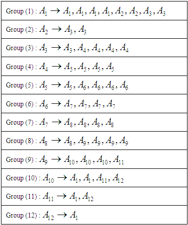
The sixth step represents the construction of groups (sums) of fuzzy relationships: that all the fuzzy relationships that were found can be grouped into a group of different fuzzy relationships according to the same left side of the fuzzy relationship. From Table (5.5.2) above, we see that the fuzzy group has a fuzzy relationship with more than one group. One, the groups are merged or combined on the right side, and no fuzzy group can appear on the right side for more than one time only, so the first group is

So,

Group (1):

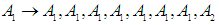And the second group is

Group (2):

And Third group is

Group (3):

And fourth group is

Seventh and final step is to raise the fuzziness to find the results of the forecast, and this step depends on the previous step.

From the first group

In this group we can find the value by Partitions middle.

Contains mid intervals of U partitions table 5.4.1.

Forecasting value Example: 606.25*0 "of A1"+1218.75*0 "of A2"+ 1831.25*0 "of A3"+...+ 7343.75*0 "of A12"=6044. This forecasted value looks much greater than the real value in Jan-2016 = 453, 09. That's why the suggested method proposes to adjust these values. We will see the full suggested method in the next section high accurate more than this method and previous method.

Table 5.5.3 and Table 5.5.4 below show the actual and forecasted values of production and consumption electric for period from January 2016 to December 2019 in GWh the result has been rounded to the nearest integer.

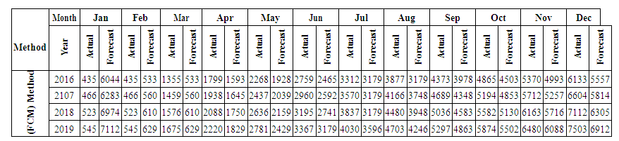Table 5.5.3. Actual and forecasted values of production electric in GWh

Table 5.5.4. Actual and forecasted values of consumption electric in GWh

5.6. Result Suggested Method for Predicting Using (FCM) and Discussion

The working steps for this model are similar to the methodology steps for the model Fuzzy c-mean method, and by using new membership function for the first order.

The first step is to define the data set. The second step is to determine the number of clusters and find the group of each the sixth and final step is to raise the fuzziness to find the program, the twelve clusters and its contents were determined from the data from January 2015 to December 2016 because we use time-invariant fuzzy time series see section 3 in this step the data will be classified based on the primes and even numbers, so that the primes and the even numbers are arranged respectively, and the results were as shown in Table (5.6.1) below:

Table 5.6.1. Clusters and fuzzy sets

The third step represents data fuzzfied this step is done by selecting each cluster as a fuzzy group, meaning that it is

We see that the third value falls within the second cluster, and accordingly it is fuzzfied. The fourth value falls within

The third cluster and so on for the rest of the data, as in Table (5.6.1) above.

The fourth step is distinguishing fuzzy relationships: From the definition of fuzzy relationships, we can extract the relationships between fuzzy groups; the following table (5.6.2) shows the fuzzy relationships.

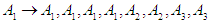
The sixth step represents the construction of groups (sums) of fuzzy relationships: that all the fuzzy relationships that were found can be grouped into a group of different fuzzy relationships according to the same left side of the fuzzy relationship. From Table (5.6.2) below, we see that the fuzzy group has a fuzzy relationship with more than one group. One, the groups are merged or combined on the right side, and no fuzzy group can appear on the right side for more than one time only, then Relationships group promises to be formed by the proposed relationship

Table 5.6.2. Fuzzy Relation Group sets

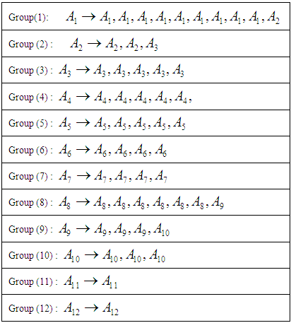
So we had the relationships

So the first group is

So,

Group (1):

And the second group is

Group (2):

And Third group is

Group (3):

Seventh and final step is to raise the fuzziness to find the results of the forecast, and this step depends on the previous step.

From the first group:

In this group we can find the value by Partitions middle,

Contains middle intervals of U partitions table 5.4.1.

Forecasting value Example: 606.25*8/9 "of A1"+1218.75*1/9 "of A2"+ 2925*0 "of A3"+...+ 7125*0 "of A12"=563.5059. This forecasted value looks near.

The real value in Jan-2016 = 453, 09. Here in this method we calculated based on different time that mean we calculate the forecast by looking to January of year 2015 That's we see the suggested method most near from the real value.

Table 5.6.3 and Table 5.6.4 below show the actual and forecasted values of production and consumption electric for period from January 2016 to December 2019 in GWh the result has been rounded to the nearest integer.

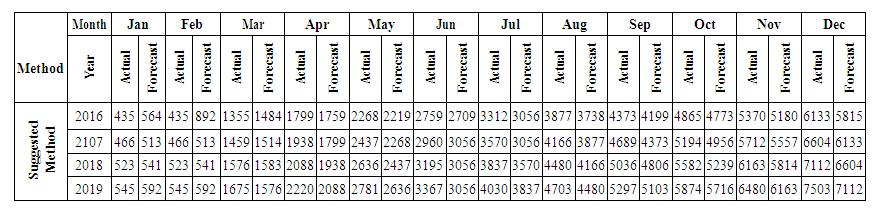Table 5.6.3. Actual and forecasted values of production electric in GWh

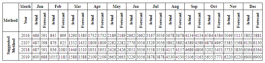Table 5.6.4. Actual and forecasted values of consumption electric in GWh

6. Conclusions

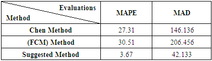
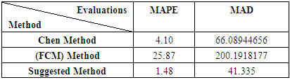
The forecasts obtained utilizing Chen method and Fuzzy Time Series c-means and Suggested Method is discussed in this paper.

The aforementioned methods require only the historical data series of electricity production and consumption to build the forecast. This can be considered as an important advantage, because the effort and cost linked to the data mining are very limited. These historical time series data are analyzed to understand the past and predict the future. Mean Absolute Percentage Error the mean absolute deviation.

The results of predictive metrics of electricity production indicated that the Mean Absolute Percentage Error ranged from 3.67 (Suggested Method) to 30.51 Fuzzy Time Series c-means and mean absolute deviation ranged from 42.133 (Suggested Method) to 146.136 Chen method.

Chen Method performed closed to the Suggested Method but Fuzzy Time Series c-means deviated a lot (Table 6.1), (Table 6.2). So, this criterion clearly indicated the superiority of Suggested Method in forecasting the production of electricity and consumption electric during 2016-2019. Similarly, the Suggested Method gave the lowest value thus performed best followed more than Chen method and Fuzzy Time Series c-means. Fuzzy Time Series c-means performed the worst in all cases.

Table 6.1. The values of evaluation metrics production of electricity

Table 6.2. The values of evaluation metrics the consumption of electricity

Similar to the prediction of electric energy production, Suggested Method performed best when the consumption of electric energy was predicted. But it is quite interesting that in case of forecasting the electric energy consumption we see from the result and discussing using time-invariant fuzzy time series better than use time-variant fuzzy time series for prediction.

This paper compared several methods to forecast production and consumption electric energy for the period of 2016 to 2019. This study has fulfilled the objectives of the study to propose the production and consumption of future electricity by different forecasting methods like Chen method and Fuzzy Time Series c-means and Suggested Method, and then inspect the accuracy of both models in forecasting ability.

After examining several models, it was found that Suggested Method was the best and most appropriate to apply to study data series of production and consumption electricity. By analyzing the forecasted value using the performance evaluation procedure, it is found that use of Suggested Method for forecasting production and consumption electricity is better Chen method and Fuzzy Time Series c-means.

Figure 3 and figure 4 shows how the actual and forecasted values too close, this is indicate we can predict for next years but the important step the chosen data and use different times, most researches No such studies shed light.

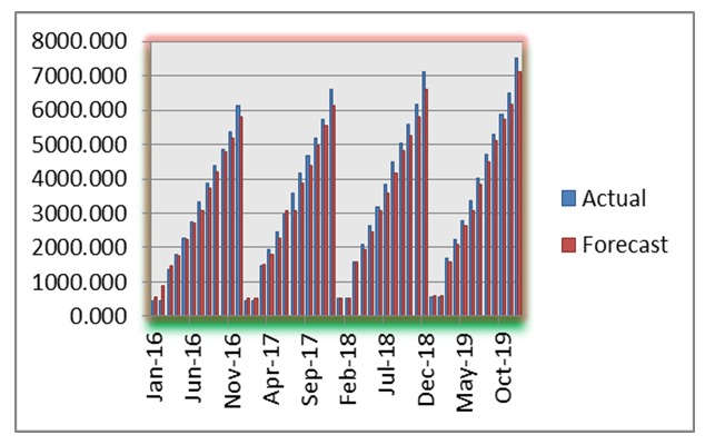Figure 3. Actual and forecasted values of Suggested Method for production electric

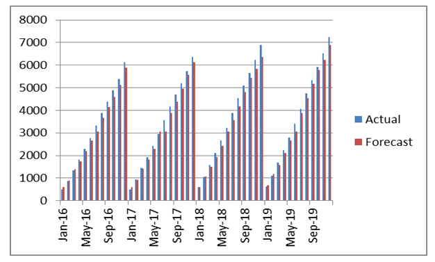Figure 4. Actual and forecasted values of Suggested Method for consumption electric