Onyekachi Akuoma Mabel, Olanrewaju Samuel Olayemi
Department of Statistics, University of Abuja, Abuja, FCT, Nigeria
Correspondence to: Olanrewaju Samuel Olayemi, Department of Statistics, University of Abuja, Abuja, FCT, Nigeria.
| Email: |  |
Copyright © 2020 The Author(s). Published by Scientific & Academic Publishing.
This work is licensed under the Creative Commons Attribution International License (CC BY).
http://creativecommons.org/licenses/by/4.0/

Abstract
This study aims to draw attention to the best extraction technique that may be considered when using the three of the most popular methods for choosing the number of factors/components: Principal Component Analysis (PCA), Maximum Likelihood Estimate (MLE) and Principal Axis Factor Analysis (PAFA), and compare their performance in terms of reliability and accuracy. To achieve this study objective, the analysis of the three methods was subjected to various research contexts. A Monte Carlo method was used to simulate data. It generates a number of datasets for the five statistical distribution considered in this study: The Normal, Uniform, Exponential, Laplace and Gamma distributions. The level of improvement in the estimates was related to the proportion of observed variables and the sum of the square loadings of the factors/components within the dataset and across the studied distributions. Different combinations of sample size and number of variables over the distributions were used to perform the analysis on the three analyzed methods. The generated datasets consist of 8 and 20 variables and 20 and 500 number of observations for each variable. 8 and 20 variables were chosen to represent small and large variables respectively. Also 20 and 500 sample sizes were chosen to represent also the small and large sample sizes respectively. The result of analysis, from applying the procedures on the simulated data set, confirm that PC analysis is overall most suitable, although the loadings from PCA and PAFA are rather similar and do not differ significantly, though the principal component method yielded factors that load more heavily on the variables which the factors hypothetically represent. Considering the above conclusions, it would be natural to recommend the use of PCA over other extraction methods even though PAF is somehow similar to its methods.
Keywords:
Principal component analysis, Maximum Likelihood, Principal Axis, Factor Analysis
Cite this paper: Onyekachi Akuoma Mabel, Olanrewaju Samuel Olayemi, A Comparison of Principal Component Analysis, Maximum Likelihood and the Principal Axis in Factor Analysis, American Journal of Mathematics and Statistics, Vol. 10 No. 2, 2020, pp. 44-54. doi: 10.5923/j.ajms.20201002.03.
1. Introduction
The origin of factor analysis dated back to a work done by Spearman in 1904. At that time Psychometricians were deeply involved in the attempt to suitably quantify human intelligence, and Spearman’s work provided a very clever and useful tool that is still at the bases of the most advanced instruments for measuring intelligence. Spearman was responsible for the development of Two-Factor Theory, in which each variable receives a contribution from two factors, a general factor common to all variables and a specific factor unique to itself. Pearson developed the methods of principal axes, later to be extended by Hotelling to become the theory of principal components. Spearman’s Two-Factor Theory was eventually superseded by multiple factor analysis in which several common or group factors are postulated and in which the specific factors are normally absorbed into the error term. From this standpoint Spearman’s Two-Factor Theory may be regarded as a one-factor theory, that is one common or group factor. For example, an individual’s response to the questions on a college entrance test is influenced by underlying variables such as intelligence, years in school, age, emotional state on the day of the test, amount of practice taking tests, and so on. The answers to the questions are the observed variables. The underlying, influential variables are the factors.The factor procedure performs a variety of common factor and component analyses and rotations. Input can be multivariate data, a correlation matrix, a covariance matrix, a factor pattern, or a matrix of scoring coefficients. The procedure can factor either the correlation or covariance matrix, and most results can be saved in an output data set. Factor analysis is used in many fields such as behavioural and social sciences, medicine, economics, and geography as a result of the technological advancements of computers.The methods for factor extraction in FA are principal component analysis, principal factor analysis, principal axis factor analysis, unweighted least-squares factor analysis, maximum-likelihood (canonical) factor analysis, alpha factor analysis, image component analysis, and Harris component analysis. A variety of methods for prior communality estimation is also available but, in this study, only the principal factor analysis, the maximum likelihood factor analysis and Principal Axis Factor analysis will be considered.Also, there are different methods for factor rotation. The methods for rotation are varimax, quartimax, parsimax, equamax, orthomax with user-specified gamma, promax with user-specified exponent, Harris-Kaiser case II with user-specified exponent, and oblique Procrustean with a user-specified target pattern. Here also, varimax will be considered further in this study.
1.1. Aims and Objectives
The main aim of this study to provide researchers with empirical derivation guidelines for conducting factor analytic studies in complex research contexts. To enhance the potential utility of this study, the researchers focused on factor extraction methods commonly employed by social scientists; these methods include principal component analysis, maximum likelihood method and principal axis factor analysis method. To meet the goal of this study, factor extraction models were subjected to several research conditions. These contexts differed in sample sizes, number of variables and distributions. Data were simulated under 1000 different conditions; specifically, this study employed a two (sample size) by two (number of variables) by five distributions.The following are the specific objectives of the study:(i) To generate artificial sample independent from each of the five distribution.(ii) To know how well the hypothesized factors explain the observed data. (iii) To determine the best extraction method in factor analysis.(iv) To compare the Principal Components Analysis, Maximum Likelihood Factor Analysis, and Principal Axis Factor Analysis method of extractions with varimax rotation method.
1.2. Theoretical Framework
1.2.1. The Orthogonal Factor Model
The aim of factor analysis is to explain the outcome of p variables in the data matrix  using fewer variables, called factors. Ideally all the information in
  can be reproduced by a smaller number of factors. These factors are interpreted as latent (unobserved) common characteristics of the observed
  . Let
. Let  be the variables in population with mean,
 and variance,
  The orthogonal factor model is
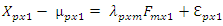 | (2.1) |
Key Concepts• F is latent (i.e. unobserved, underlying) variable • X’s are observed (i.e. manifest) variables•  is measurement error for Xj.•
  is the “loading” for Xj.
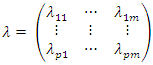 is called the factor loading matrix
 are called the factors or common factors,
 are called errors or specific errors.This is written in matrix notation as
 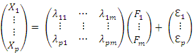 Our hypothesis is that these values arise from a linear combination of k factors,
  plus noise,
  The model can be re-expressed as
 | (2.2) |
And  is called the loading of
  on the factor
  In the factor Matrix
 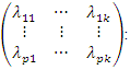 • Columns represent derived factors. • Rows represent input variables. • Loadings represent degree to which each of the variable “correlates” with each of the factors •Loadings range from -1 to 1.• Inspection of factor loadings reveals extent to which each of the variables contributes to the meaning of each of the factors. • High loadings provide meaning and interpretation of factors (regression coefficients).
1.2.2. Review of Previous Studies
For this research work, different related theses, websites, books, journals, articles etc. have been studied, it is discovered that John Spearman was first to find the use of Factor Analysis in developing psychology and sometimes credited with the invention of factor analysis. He discovered that school children study on variety of seemingly unrelated subjects which are positively correlated. This led him to postulate that the General Mental Ability (GMA) underlies and shapes human cognitive performance. This postulate now enjoys broad support in the field of intelligence research which is known as the G-theory.Raymond Cattel expanded on Spearman’s idea of a two-factor theory of intelligence after performing his own tests on factor analysis. He used a multi-factor theory to explain intelligence. Cattell’s theory addressed alternate factors in intellectual development, including motivation and psychology. Cattell also developed several mathematical methods for adjusting psychometric graphs such as his “scree” test and similarity coefficients. His research led to the development of his theory of fluid and crystallized intelligence as well as his sixteen (16) personality factors theory of personality.[1] examined the information reported in 60 exploratory factor analyses published before 1999. The authors focused on studies that employed at least one exploratory factor analysis strategy. Although Henson and Roberts noted that most of the articles reported researcher objectives that warranted an EFA design, nearly 57% of the researchers engaged in principal components analysis. As a suggested rationale for this problematic model selection, the authors noted that principal components analysis was the “default option for most statistical software packages” ([1]). The goal for factor retention guidelines is to identify the necessary number of factors to account for the correlations among measured variables. Empirical research suggests that under-factoring, retaining too few factors, is more problematic than over- factoring ([2]). However, over-factoring is not ideal; for example, when over-factoring, researchers may postulate the existence of factors with no theoretical basis which can “accentuate poor decision made at other steps in factor analysis” ([2]).Orthogonal rotation algorithms yield uncorrelated factors ([2]; [3]; [4]). The most commonly employed type of orthogonal rotation is varimax ([2]). Although orthogonal rotation yields simple structure, the use of orthogonal rotation when the factors are correlated in the population results in the loss of important data ([5]).In published literature, orthogonal strategies appear to be the most commonly cited rotation procedure. According to [6] findings, researchers reported using an orthogonal rotation strategy most frequently (40%); in only 18% of the studies, researchers reported the use of an oblique rotation strategy. More recently, in their study of common practices in factor analytic research, [1] found that 55% of the articles included orthogonal rotation strategies; researchers reported the use of oblique rotation strategies in 38.3% of the articles, and, in 1.7% of the articles, researchers failed to report any factor rotation method.The “conventional wisdom advises researchers to use orthogonal rotation because it produces more easily interpretable results . . .” ([5]). However, this argument is flawed in two areas. Firstly, social science researchers “generally expect some correlation among factors” ([5]); therefore, the use of orthogonal rotation results in the loss of information concerning the correlations among factors. Secondly, output associated with oblique rotation is “only slightly more complex” than orthogonal rotation output and yield substantive interpretations that “are essentially the same” ([5]).[7] in his book, Robustness of the Maximum Likelihood Estimation procedure in factor analysis, generated random variables from six distributions independently on a high-speed computer and then used to represent the common and specific factors in a factor analysis model in which the coefficients of these factors had been specified. Using Lawley's approximate χ2 statistic in evaluating the estimates obtained, the estimation procedure is found to be insensitive to changes in the distributions considered.A Monte Carlo Study Comparing Three Methods for Determining the Number of Principal Components and Factors by [7] was conducted. The results of the analysis confirm the findings from previous papers that Kaiser criterion has the poorest performance compared with the other two analyzed methods. Parallel analysis is overall the most accurate, although when the true number of factors/ components is small, acceleration factor can outperform it. The acceleration factor and Kaiser criterion perform with different accuracy for different true number of factors/ components and number of variables, whereas the parallel analysis is only affected by the sample size. Kaiser criterion tends to overestimate and acceleration factor – to underestimate the number of factors/ components. The parallel analysis shows fewer fluctuations in its accuracy and is more robust. [8] conducted a research on the Principal component procedure in factor analysis and robustness. In her study she said that Principal component procedure has been widely used in factor analysis as a data reduction procedure. The estimation of the covariance and correlation matrix in factor analysis using principal component procedure is strongly influenced by outliers. The study investigated the robustness of principal component procedure in factor analysis by generating random variables from five different distributions which are used to determine the common and specific factors in factors analysis using principal component procedure. The results revealed that the variance of the first factor was widely distributed from distribution to distribution ranging from 0.6730 to 5.9352. The contribution of the first factor to the total variance varied widely from 15 to 98%. It was therefore concluded that the principal component procedure is not robust in factor analysis.In the book, Exploratory Factor Analysis by [2] summarizes the key issues that researchers need to take into consideration when choosing and implementing exploratory factor analysis (EFA) before offering some conclusions and recommendations to help readers who are contemplating the use of EFA in their own research. It reviews the basic assumptions of the common factor model, the general mathematical model on which EFA is based, intended to explain the structure of correlations among a battery of measured variables; the issues that researchers should bear in mind in determining when it is appropriate to conduct an EFA; the decisions to be made in conducting an EFA; and the implementation of EFA as well as the interpretation of data it provides.Robustness of the maximum likelihood estimation procedure in factor analysis by [9] is that of random variables generated from five distributions which were used to represent the common and specific factors in factor analysis in order to determine the robustness of the maximum likelihood estimation procedure. Five response variables were chosen for this study each with two factors. The chosen variables were transformed into linear combinations of an underlying set of hypothesized or unobserved components (factors). The result revealed that the estimates of the variance for the first factor were found to be almost the same and closely related to each other in all the distributions considered. The Chi-Square test conducted concluded that maximum likelihood method of estimation is robust in factor analysis.[10] wrote on a robust method of estimating covariance matrix in multivariate data analysis. This is also a research paper where a proposed robust method of estimating covariance matrix in multivariate data set was done. The goal was to compare the proposed method with the most widely used robust methods (Minimum Volume Ellipsoid and Minimum Covariance Determinant) and the classical method (MLE) in detection of outliers at different levels and magnitude of outliers. The proposed robust method competes favorably well with both MVE and MCD and performed better than any of the two methods in detection of single or fewer outliers especially for small sample size and when the magnitude of outliers is relatively small.
2. Methodology
2.1. Research Design
The research method used in this study is Monte Carlo design to generate a data set. This incorporated samples simulated through different number of variables and sample sizes; specifically, a two (number of variables) and two (sample size) by five (distributions) design.
2.2. Population of the Study
This simulation was developed in RGUi (64 – bit). The program associated with this design was written. To enhance this project’s generalizability, this study included simulations of results from data sets of varying size. It simulated data sets containing 8 and 20 variables. The two sample sizes included in this study were 20 (small sample size) and 500 (large sample size). The initial factor solutions from each model in each condition was subjected to an orthogonal rotation strategy. Specifically, this study employed a varimax rotation in all simulated contexts. Because the intent of this study is to address methodological issues that are frequently encountered in social science literature, varimax rotation was considered to be a more appropriate choice ([2]; [11]).
2.3. Sample Size and Sampling Procedure
Determining the sample size is a very important issue in factor analysis because samples that are too large may waste time, resources and money, while samples that are too small may lead to inaccurate result. Larger samples are better than smaller samples (all other things being equal) because larger samples tend to minimize the probability of errors, maximize the accuracy of population estimates, and increase the generalizability of the results. Factor analysis is a technique that requires a large sample size. Factor analysis is based on the correlation matrix of the variable involved and correlations usually need a large sample size before they stabilize. [12] suggested that “the adequacy of sample size might be evaluated very roughly on the following scale: 50 – very poor; 100 – poor; 200 – fair; 300 – good; 500 – very good; 1000 or more – excellent” (p. 217). It is known that a sample size of 200 or more is sufficient for a sample number of independent variables. As the sample size gets larger for Maximum Likelihood Estimator, the estimates become consistent, efficient and unbiased. So in our experiment, we will consider two types of sample sizes – 20 (small) and 500 (large) sample number of independent variables.
2.4. Instrumentation/Factor Extraction Method
Maximum likelihood factoring allows the researcher to test for statistical significance in terms of correlation among factors and the factor loadings, but this method for estimating factor models can yield distorted results when observed data are not multivariate normal ([5]; [1]). Principal axis factoring does not rely on distributional assumptions and is more likely than maximum likelihood to converge on a solution. However, principal axis factoring does not provide the variety of fit indices associated with maximum likelihood methods, and this method does not lend itself to the computation of confidence intervals and tests of significance.Consider a data vector for subject i on p variables represented as:  Standardization of the data matrix X is performed since the p variables could be in different units of measurement. The standardized matrix, Z, is written as Z = (V1/2)-1 (X - µ), where V1/2 is the diagonal standard deviation matrix and µ is the vector of the means. Clearly, E(Z) = 0 and Cov(Z) = (V 1/ 2 )-1 (V 1/ 2 ) = ρ, where ∑ is the variance-covariance matrix and is the population correlation matrix. The kth principal component of Z =(Z1 Z2 ... Z p )/ is given by:
  | (3.1) |
where (λk, ek) is the kth eigenvalue-eigenvector pair of the correlation matrix, with λ1 ≥ λ2 ≥...≥λp ≥0. Since Zi is a standardized variable,  and the correlation coefficient between component Yk and standardized variable Zl is
 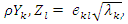 k, l = 1, 2, …, p. The proportion of standardized population variance due to the kth principal component is λk/ p.A correlation matrix can be thought of as a matrix of variances and covariances of a set of variables that have standard deviations of 1. It can be expressed as a function of its eigen values λk and eigenvectors, ek, as follows:
 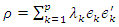 | (3.2) |
The correlation matrix is modeled as ρ = LL’ + Ψ, where Ψ is a diagonal matrix of specific variances. As a principal component analysis takes all variance into account, Ψ is assumed to be zero and the variance-covariance matrix is modeled as ρ = LL’. A PCA procedure will try to approximate the correlation by a summation over m<p, i.e. 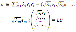 | (3.3) |
where L is the matrix of factor loadings with a factor loading estimated as  .
.
2.5. Data Collection Procedure
2.5.1. Extraction by Principal Component Analysis Method
The principal factor method involves finding an approximation  the matrix of specific variances, and then correcting R, the correlation matrix of
  The principal component method is based on an approximation
  the factor loadings matrix. The sample covariance matrix is diagonalized,
  . Then the first
  eigenvectors are retained to build
  The estimated specific variances are provided by the diagonal elements of the matrix
 By definition, the diagonal elements of
  are equal to the diagonal elements of
 The off-diagonal elements are not necessarily estimated. How good then is this approximation? Consider the residual matrix
 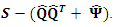 resulting from the principal component solution. Analytically we have that
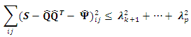
2.5.2. Extraction by Maximum Likelihood Factor Analysis
In finding factors that can reproduce the observed correlations or covariances between the variables as closely as possible, a maximum likelihood estimation (MLE) procedure will find factors that maximize the likelihood of producing the correlation matrix. In trying to do so, it assumes that the data are independently sampled from a multivariate normal distribution with mean vector µ, and variance-covariance matrix of the form  where L is the matrix of factor loadings and Ψ, is the diagonal matrix of specific variances. The MLE procedure involves the estimation of µ, the matrix of factor loadings L, and the specific variance Ψ, from the log likelihood function which is given by the following expression:
  By maximizing the above log likelihood function, the maximum likelihood estimators for µ, L and Ψ are obtained.
2.5.3. Extraction by Principal Axis Factoring
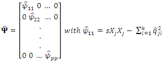
The most widely-used method of extraction in factor analysis is the principal axis factoring (PAF) method. The method seeks the least number of factors which can account for the common variance of a set of variables. In practice, PAF uses a PCA strategy but applies it on a slightly different version of the correlation matrix. As the analysis of data structure in PAF is focused on common variance and not on sources of error that are specific to individual measurements, the correlation matrix ρ in PAF has estimates of communalities as its diagonal entries, instead of 1’s as in PCA. Allowing for specific variance, the correlation matrix is estimated as 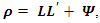 where Ψ is a diagonal matrix of specific variances. The estimate of the specific variances is obtained as
  where matrix
  is as defined in (3) and diagonal entries Ψ are estimated as
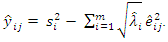
2.6. Method of Data Analysis
For this study, simulated data was used to examine the effects of (1) Principal Component Analysis, Maximum Likelihood analysis method and Principal Axis factoring method, (2) Small and large variables, (3) Small and large sample sizes using varimax on five statistical distributions: Uniform, Normal, Gamma, Exponential, and Laplace. Our goal was to utilize methods that most closely simulate real practice, and real data, so that our results will shed light on the effects of current practice in research and also advise researchers on the best extraction method that can be adopted in data analysis to accomplish their goal.
2.7. Data Presentation, Analysis and Interpretation
2.7.1. Presentation of Data
The result of the first Principal Component/Maximum Likelihood/Principal Axis Loadings from the simulation of each sample from the various distribution with respect to each extraction method is presented in the table below: 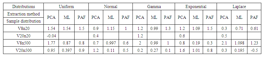 | Table 1. First Principal Component/Maximum Likelihood/Principal Axis Loadings from the simulation |
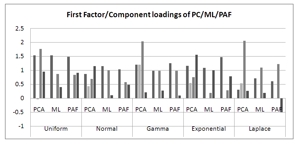 | Figure 1. First Principal Component/Maximum Likelihood/Principal Axis Loadings from the simulation |
The result of the Sum of Square loadings and Proportion Variance of the 1st principal component/Maximum Likelihood/principle axis of each sample from the various distribution with respect to each extraction method is presented in the table below: 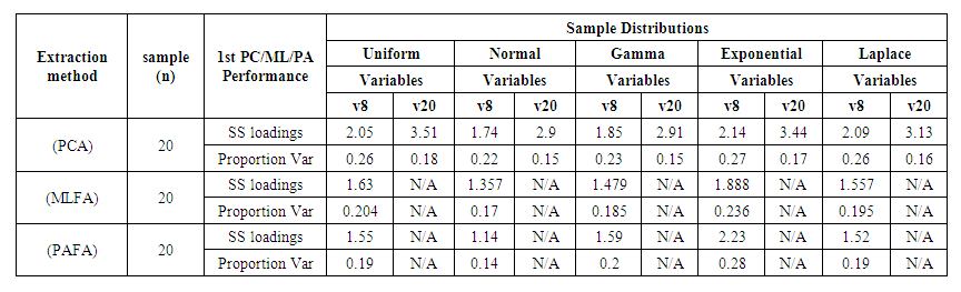 | Table 2. Simulation Results for Sample = 20 |
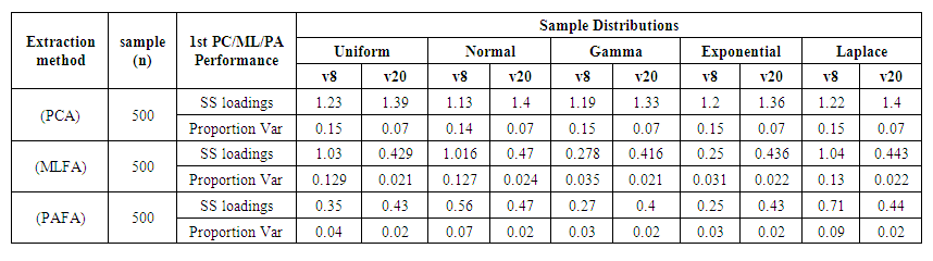 | Table 3. Simulation Results for Sample = 500 |
2.7.2. Data Analysis and Result
Factor analysis uses variances to produce communalities between variables. The variance is equal to the square of the factor loadings. In many methods of factor analysis, the goal of extraction is to remove as much common variance in the first factor as possible. From table 1, we compare the different extraction methods per each of the distribution. It was observed that:• PC is the best extraction method for Uniform distribution for all variables and all samples.• For Normal distribution, ML is the best extraction method for normal when working with 8 variables (small) over different sample sizes but PC is better when the variables are 20 (large) over large sample sizes.• For Gamma distribution, PC and PAF are better with 8 (small) variables and 20 (small) sample sizes; PC is best for 8 (small) variables and 500 (large) samples sizes while ML is better with 20 (large) variables over large sample sizes.• For Exponential distribution, all the extraction methods studied are good but PAF is the best for small variables and sample sizes while PC is the best for different variables with large numbers.• For Laplace distribution, ML and PAF are good methods to use for small variables and small sample sizes though ML performed better. PC performed better the other large variables and large sample sizes even at small variables and large sample sizes.Comparing the same number of variables and sample sizes over different distributions.Also, from table 1, we can deduce that:• For small (8) variables and small (20) number of samples, all the extraction methods can be used for analysis since the sum of the factor loading are above 0.5 across all the distributions except for PC method for Laplace distribution.• Only PC can be used for analysis when the variables have equal variables with the sample size.• For small (8) variables and large (500) sample sizes, PC formed better across all distributions except for normal distribution where ML is slightly higher but Uniform, Gamma and Laplace distributions perform best when large sample size is applied with smaller variables using PCA. • For large variables and large sample sizes, PC performed better across all the distributions.Using figure 2, when the sample size is small over small and large variables, it can be observed that for the sum of square loadings of the extraction methods across the distributions, PC is seen to perform better than other extractions methods for all variables and all distributions used in this study.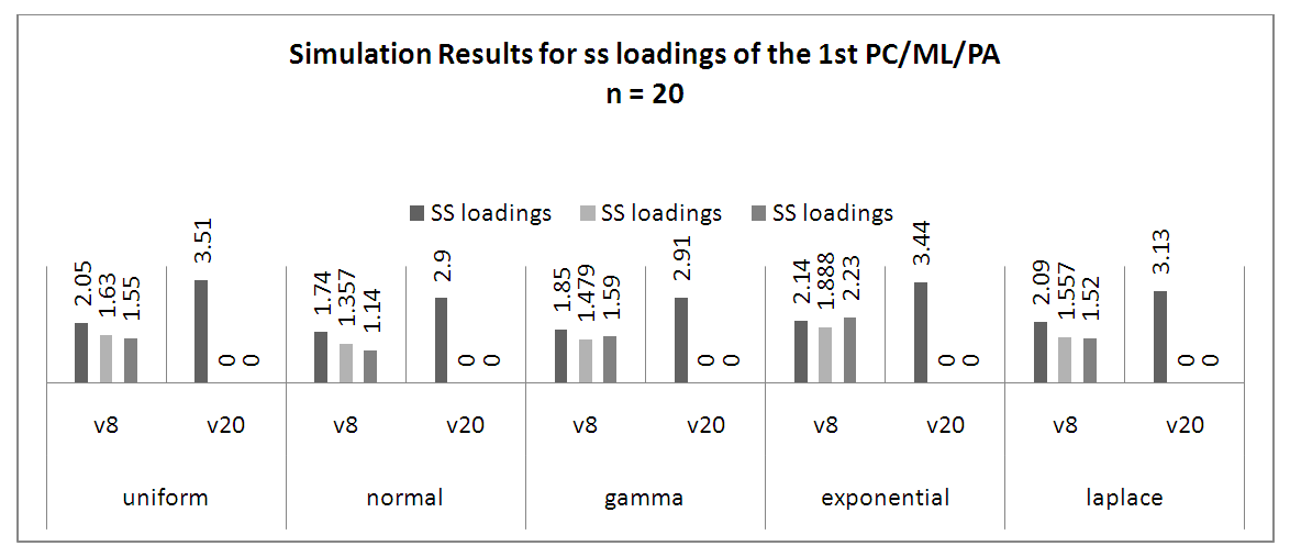 | Figure 2. Simulation Results for SS Loadings of the 1st PC/ML/PA at 20 Samples |
Figure 3 explained the proportion variance for small sample sizes over small variables, PC is the best method for all distributions. PAF explains the greatest in the Exponential distribution over others. Also, when compared other small sample sizes and small variables, PAF is seen to perform very well.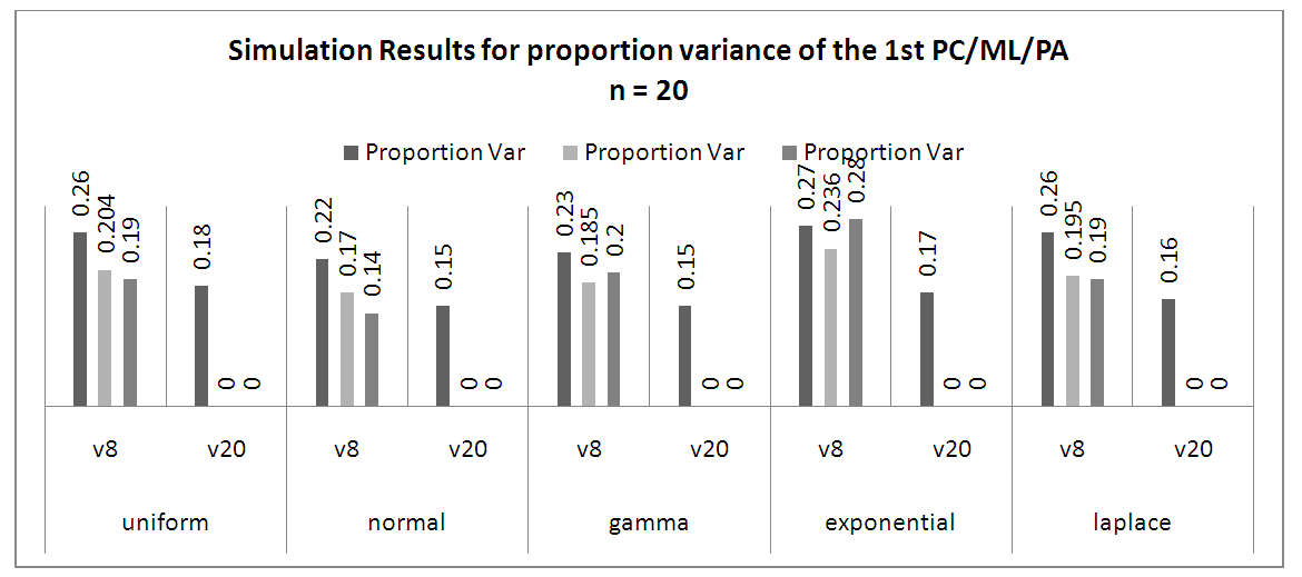 | Figure 3. Simulation Results for Proportion Variance of the 1st PC/ML/PA at 20 Samples |
In Figure 4, when the sample size is large, PC showed the highest the ssloadings for all variables over all distributions. In figure 5, for the large sample sizes, PC explained the highest proportion variance across the distribution. It was also seen that the proportion variance of the PC seems equals over all small variables and also the same across the large variables.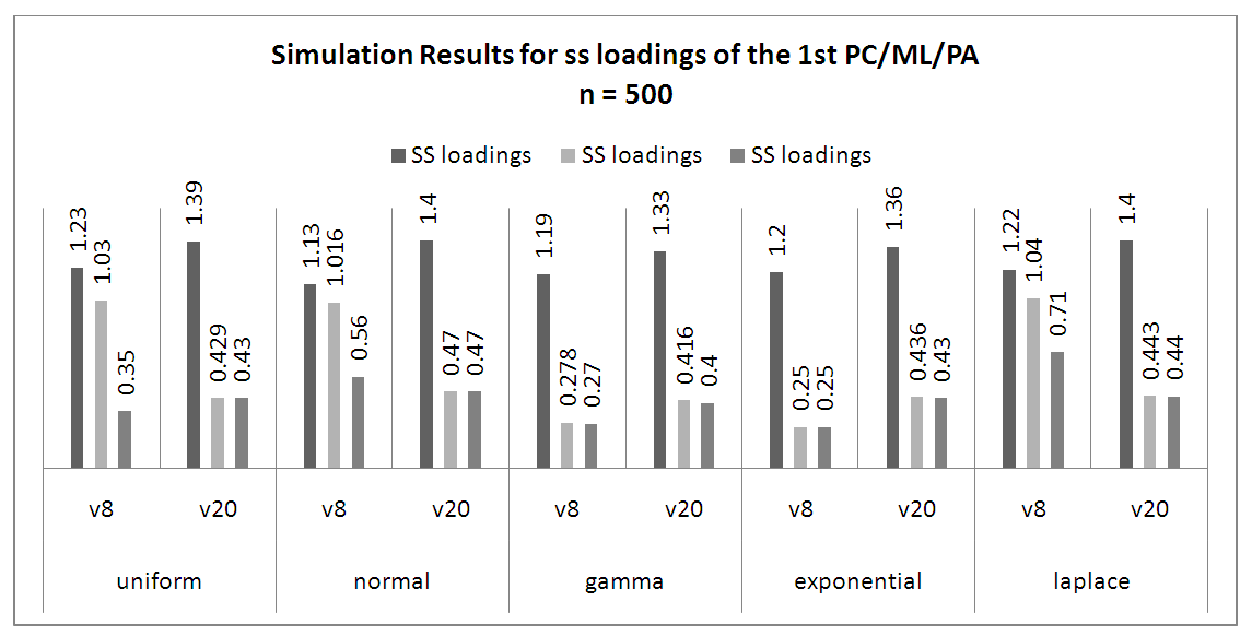 | Figure 4. Simulation Results for SS Loadings of the 1st PC/ML/PA at 500 Samples |
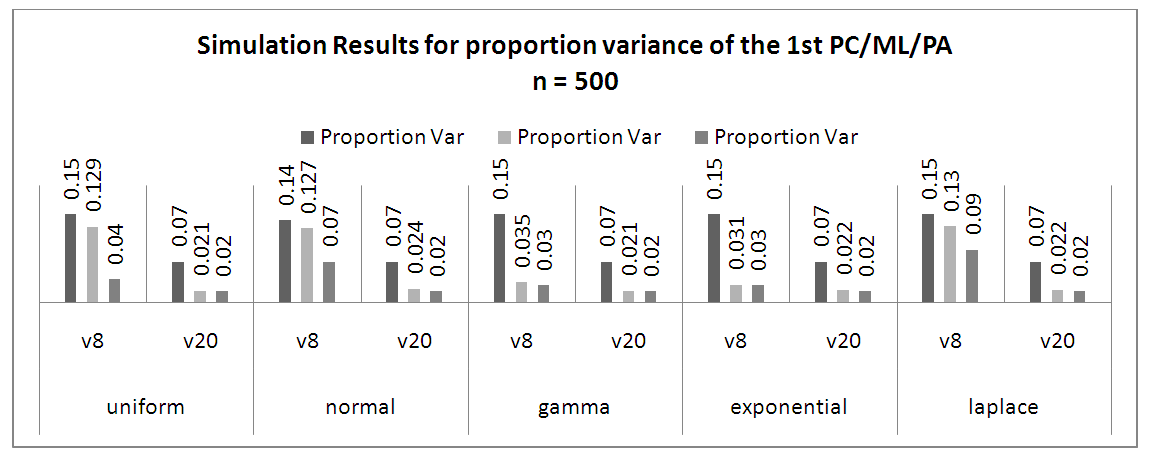 | Figure 5. Simulation Results for Proportion Variance of the 1st PC/ML/PA at 500 Samples |
Figure 6, for ss loadings across the sample sizes, PC performed better over small sample sizes than the large sample sizes. Same also it is for proportion variables as observed in figure 7.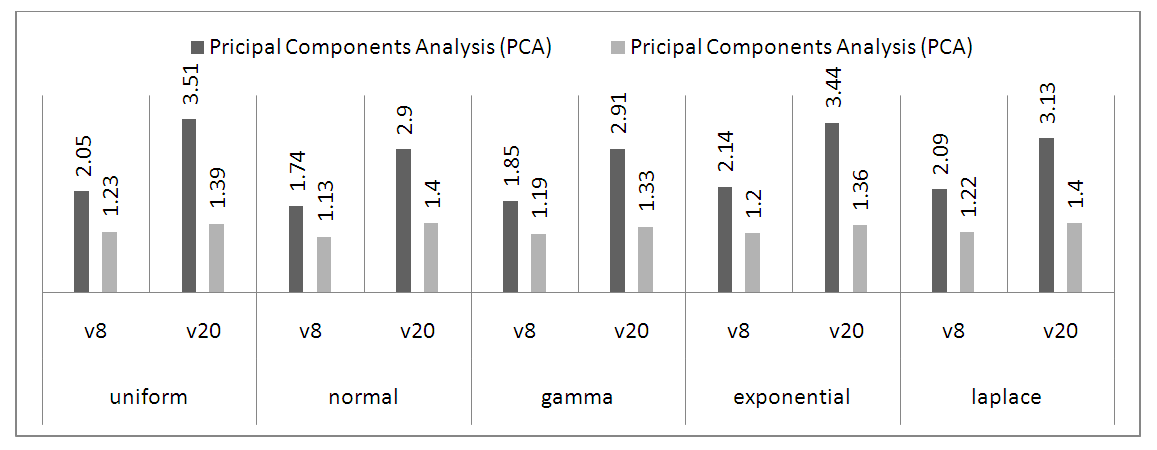 | Figure 6. Principal Component Analysis, SS Loadings for 20 and 500 samples |
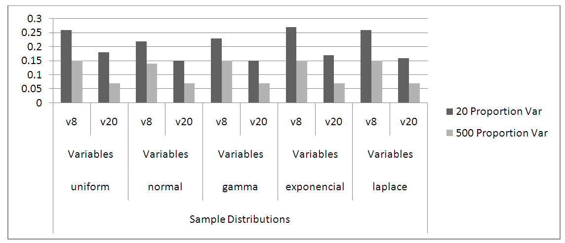 | Figure 7. Principal Component Analysis, Proportion Variances for 20 and 500 samples |
3. Discussion on Findings
From the figure 1 above, we can observe that Uniform, Gamma and Laplace distributions perform best when large sample size is applied with smaller variables using PCA. Also, the proportion of variance explained by PCA is higher on a lower variable than large variable.Similarly, when the three extractions methods were applied on a real-life data used under this study, the methods of PCA and PAF methods achieved a simple structure of the loadings following rotation. The loadings from each method are rather similar and don’t differ significantly, though the principal component method yielded factors that load more heavily on the variables which the factors hypothetically represent. However, the factors resulting from the principal component method explain 54% of the cumulative variance compared to 46% from the principal factor method.
4. Summary
The broad purpose of factor analysis is to summarize data so that relationships and patterns can be easily interpreted and understood. It is normally used to regroup variables into a limited set of clusters based on shared variance. Hence, it helps to isolate constructs and concepts.The goal of this paper is to collect information that will allow researchers and practitioners to understand the various choices of factor extractions available, and to make decisions about "best practices" in exploratory factor analysis. A Monte Carlo study has been performed for assessing the accuracy of three frequently used methods for extraction of number of factors and components in factor analysis and principal component analysis: The Principal Components Analysis, Maximum Likelihood Factor Analysis, and Principal Axis Factor Analysis method.Data was generated independently in a sequence of 1000 replications through simulation for factor analysis, so that it would have a specific number of underlying components or factors: Then the three methods for extracting the number of factors/components were applied and their overall performance examined. The SS loadings of the different distributions using different variables and sample sizes were computed as well as the proportion variance of the distribution on different extraction methods from the simulated data. The procedure was performed by simulating datasets with 8 and 20 number of variables over sample sizes of 20 and 500 for all combinations of 8 and 20 (number of variables). In summary, our research seems to agree with [2] that says that when each factor is represented by three to four measured variables and the communalities exceed .70, relatively small sample sizes will allow researchers to make accurate estimates about population parameters as observed with the real-life data set. To avoid distortions derived from sample characteristics, researchers can select a sample that maximizes variance on measured variables that are not relevant to the construct of interest ([2]).
5. Conclusions
From some of the literatures reviewed, many researchers believe that there is almost no evidence regarding which method should be preferred for different types of factor patterns and sample sizes. Some of these contributed to this research and the following conclusions can be drawn from the results, obtained by the Monte Carlo simulations: • PC is the best extraction method for Uniform distribution for all variables and all samples.• For Normal distribution, ML is the best extraction method for normal when working with 8 variables (small) over different sample sizes but PC is better when the variables are 20 (large) over large sample sizes.• For Gamma distribution, PC and PAF are better with 8 (small) variables and 20 (small) sample sizes; PC is best for 8 (small) variables and 500 (large) samples sizes while ML is better with 20 (large) variables over large sample sizes.• For Exponential distribution, all the extraction methods studied are good but PAF is the best for small variables and sample sizes while PC is the best for different variables with large numbers.• For Laplace distribution, ML and PAF are good methods to use for small variables and small sample sizes though ML performed better. PC performed better the other large variables and large sample sizes even at small variables and large sample sizes.Comparing the same number of variables and sample sizes over different distributions.Also, from table 1, we can deduce that:• For small (8) variables and small (20) number of samples, all the extraction methods can be used for analysis since the sum of the factor loading are above 0.5 across all the distributions except for PC method for Laplace distribution.• Only PC can be used for analysis when the variables have equal variables with the sample size.• For small (8) variables and large (500) sample sizes, PC formed better across all distributions except for normal distribution where ML is slightly higher but Uniform, Gamma and Laplace distributions perform best when large sample size is applied with smaller variables using PCA. • For large variables and large sample sizes, PC performed better across all the distributions.
6. Recommendations
This thesis only analyses three of the most commonly used methods for extracting the number of factors and components in FA and PCA. However, there are other developed methods such as Image Factor Extraction, Unweighted Least Squares Factoring, Generalized Least Squares Factoring and Alpha Factoring and used only in principal component analysis. A review of these methods would be a suitable continuation of the current thesis. The knowledge of studies, such as this one can help researchers pinpoint the best extraction method of number of factors or components, even if all the methods have given different estimates. To do so, one has to know the strengths and weaknesses of each method and how they compare to each other for different combinations of variables and sample sizes.
References
| [1] | Henson, R. K., & Roberts, J. K. (2006). Use of Exploratory Factor Analysis in Published Research: Common Errors and Some Comment on İmproved Practice. Educational and Psychological Measurement, 66, 393–416. |
| [2] | Fabrigar, L. R., Wegener, D. T., MacCallum, R. C., & Strahan, E. J. (1999). Evaluating the Use of exploratory factor analysis in psychological research. Psychological Methods, 4(3), 272-299. |
| [3] | Harman, H.H. (1976). Modern factor analysis (3rd ed. revised). Chicago, IL: University of Chicago Press. |
| [4] | Stevens, J. P. (2002). Applied multivariate statistics for the social sciences (4th ed.). Hillsdale, NS: Erlbaum. |
| [5] | Costello, A.B., & Osborne, J.W. (2005). Best practices in exploratory factor analysis: Four recommendations for getting the most from your analysis. Practical Assessment, Research and Evaluation, 10(7), 1-9. |
| [6] | Conway, J. M., & Huffcutt’s, A. I. (2003). A review and evaluation of exploratory factor analysis practices in organizational research. Organizational Research Methods, 6(2), 147-168. |
| [7] | Fuller E. L. & Hemmerle W. J. (1966). Robustness of the maximum-likelihood estimation procedure in factor analysis. Psychometrika, Volume 31, pp 255–266. |
| [8] | Nwabueze J. C. (2010). Principal component procedure in factor analysis and robustness. Academic. Journals 2010 TEXT text/html https://academicjournals.org/journal/AJMCSR/article-abstract/CC194D88841. |
| [9] | Nwabueze, J. C., Onyeagu, S. I. & Ikpegbu O. (2009). Robustness of the maximum likelihood estimation procedure in factor analysis. African Journal of Mathematics and Computer Science Research Vol. 2(5), pp. 081-087. |
| [10] | Oyeyemi, G.M. and Ipinyomi, R.A. (2010). Some Robust Methods of Estimation in Factor Analysis in the Presence of Outliers. ICASTOR Journal of Mathematical Sciences. Vol. 4. No.1 Pp. 1-12. |
| [11] | Raykov T. & Little T. D. (1999). A Note on Procrustean Rotation in Exploratory Factor Analysis: A Computer Intensive Approach to Goodness-of-Fit Evaluation. https://doi.org/10.1177/0013164499591004. |
| [12] | Comfrey, L.A. & Lee, H.B. (1992). A first course in factor analysis (2nd ed.). Hillside, NJ: Lawrence Erlbaum Associates. |

 Abstract
 Reference
 Full-Text PDF
 Full-text HTML