K. C. N. Dozie 1, C. C. Ibebuogu 2, H. I. Mbachu 1, M. C. Raymond 1
1Department of Statistics Imo State University Owerri, Imo State Nigeria
2Department of Computer Science Imo State University Owerri, Imo State, Nigeria
Correspondence to: K. C. N. Dozie , Department of Statistics Imo State University Owerri, Imo State Nigeria.
| Email: |  |
Copyright © 2020 The Author(s). Published by Scientific & Academic Publishing.
This work is licensed under the Creative Commons Attribution International License (CC BY).
http://creativecommons.org/licenses/by/4.0/

Abstract
This study presents time series analysis on a method of modeling the church marriages in time series decomposition, when trend-cycle component is linear. Empirical example was drawn from monthly records of number of church marriages in Imo State, Nigeria over the period of January, 1997 to December, 2016. The ultimate objective of this study is therefore, to determine the appropriate model of the monthly number of church marriages over the period under investigation. The method adopted is Buys-Ballot procedure developed for choice of model and choice appropriate transformation, among other uses, based on row, column and overall means and variances of the Buys-Ballot table. Result from the test shows that, the appropriate model of original data is multiplicative. The test requires that the study series satisfies the assumptions of the time series model.
Keywords:
Time Series Decomposition, Data Transformation, Choice of Model, Buys-Ballot table
Cite this paper: K. C. N. Dozie , C. C. Ibebuogu , H. I. Mbachu , M. C. Raymond , Buys-Ballot Modeling of Church Marriages in Owerri, Imo State, Nigeria (1997-2016), American Journal of Mathematics and Statistics, Vol. 10 No. 1, 2020, pp. 26-31. doi: 10.5923/j.ajms.20201001.04.
1. Introduction
Three models commonly used in time series date are additive, multiplicative and mixed models.If short period of time are involved, the trend component is superimposed into the cyclical Chatfield [3] and the observed time series  can be decomposed into the trend-cycle component
  , seasonal component
  and the irregular component
  . Therefore, the decomposition models areAdditive Model:
  | (1) |
Multiplicative Model:  | (2) |
and Mixed Model  | (3) |
As far as the descriptive method of decomposition is concerned, the first step will usually be to estimate and eliminate trend-cycle  for each time period from the actual data either by subtraction, for Equation (1) or division, for Equation (2). The de-trended series is obtained as
  for Equation (1) or
  for Equations (2) and (3). The seasonal effect is obtained by estimating the average of the de-trended series at each season. The de-trended, de-seasonalized series is obtained as
  for Equation (1) or
  for Equations (2) and (3). This gives the residual or irregular component. Having fitted a time series model, one often wants to see if the residuals are purely random. For details of residual analysis, see Box, et al, [2] and Ljung and Box [7]. It is always assumed that the seasonal effect, when it exists, has period s, that is, it repeats after s time periods.
 | (4) |
For Equation (1), it is assumed to make the further assumption that the sum of the seasonal components over a complete period is zero, ie, | (5) |
Similarly, for Equations (2) and (3), it is also assumed to make further assumption is that the sum of the seasonal components over a complete period is s. | (6) |
In all the steps outlined above, it is assumed that (i) the appropriate model for decomposition is known; (ii) the study series satisfied the assumptions of the models and (iii), all the components of time series may or may not exist in a study series. However, one of the greatest challenges identified in the use of descriptive method of time series analysis is choice of appropriate model for decomposition of any study data. That is when to use any of the three models for analysis is uncertain. And it is important to note that; wrong use of model will definitely lead to erroneous estimates of the components.To choose between additive and multiplicative models. Chatfield [3] observed that, if the seasonal variation is independent of the absolute level of the time series, but it takes approximately the same magnitude each year then the appropriate model is additive and for the multiplicative model, the seasonal changes increase with the overall trend. Linde [6] stated the difference between additive and multiplicative models. In his opinion, if the seasonal variation is independent of the absolute level of the time series, but it takes appropriately the same magnitude each year then the appropriate model is additive. For multiplicative model, the seasonal variation takes the same relative magnitude each year. Iwueze, et al, [5] gave five uses of the Buys-Ballot table in time series analysis including 1) choice of appropriate model for time series decomposition. 2) choice of appropriate transformation 3) estimation of trend parameters and seasonal indices. They proposed the use of the relationship between the seasonal means  and the seasonal standard deviations
  to choose the appropriate model for decomposition. An additive model is appropriate when the seasonal standard deviations show no appreciable increase or decrease relative to any increase or decrease in the seasonal means. On the other hand, a multiplicative model is usually appropriate when the seasonal standard deviations show appreciable increase/decrease relative to any increase /decrease in the seasonal means. Oladugba, et al, [9] gave brief description of additive and multiplicative seasonality. According to them, the seasonal fluctuation exhibits constant amplitude with respect to the trend in additive case while amplitude of the seasonal fluctuation is a function of the trend in multiplicative seasonality.
1.1. Choice of Appropriate Transformation
Transformation is a mathematical operation that changes the measurement scale of a variable. Many scholars have stated different reasons for transformation, which include stabilizing variance, normalizing, reducing the effect of outlines, making measurement scale more meaningful and linearizing a relationship. Many of these time series analyst assume normality and it is well known that variance stabilization implies normality of the series. According to Chatfield [3], if there is a trend in the series and the variance appears to increase with mean, then it may be necessary to transform the data particularly, if the standard deviation is directly proportional to the mean, a logarithmic transformation is indicated. The emphasis of this study is to explore the appropriate transformation that will be suitable for the analysis of church marriages Owerri, Imo State, Nigeria, between 1997 -2016 and to ensure that, the met some appropriate inference procedure. In the analysis of this time series data under the descriptive approach. The ultimate objective of this study is there, to determine the appropriate the model of the monthly number of church marriages over the period under investigation.
1.2. Review of Buys-Ballot Procedure
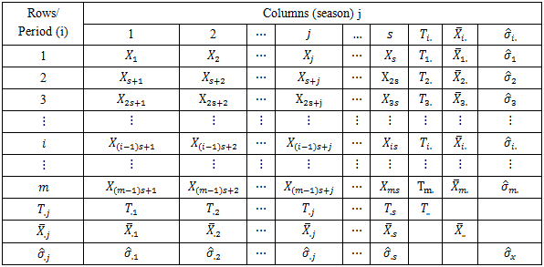
Iwueze, et al, [5] highlighted seasonal variation (Table 1) of the Buys - Ballot table. Each row is one period (usually a year) and each column is a season of the period/year (4 quarter, 12 months etc). A cell,  of the table contains the mean value for all observations made during the period
  at the season
  To analyse the data, it is important to include the period and seasonal totals
  and
and  period and seasonal averages
  and
and  period and seasonal standard deviations
  and
and  as part of the Buys – Ballot table. Also, included for purposes of analysis are the grand total
  grand mean
  and pooled standard deviation
  Chatfield [2] proposed that, the Buys - Ballot table is used for inspecting time series data for the presence of trend and seasonal effect Iwueze and Nwogu [4] suggested a new estimation method based on row, column and overall averages of the Buys - Ballot table. According to them, the method called Buys – Ballot estimation procedure uses the periodic mean
  and the overall mean
  to estimate the trend component. Seasonal means
  and the overall mean
  are used to estimate the seasonal indices.
Table 1. Buys - Ballot Table for Seasonal time series
 |
| |
|
In this arrangement each time period t is represented in terms of the period i (e.g. year) and season j (e.g. month of the year), as  Thus, the period (row), season (column) and overall totals, means and variances are defined as
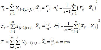
2. Proposed Chi-square Test
Nwogu, et al, [8] proposed a test for choice between mixed and multiplicative models that can be based on the seasonal variances of the Buys-Ballot table. Test is able to distinguish the series that admits mixed model from the series that admits multiplicative model. It is clear that, the mixed model is a constant multiple of square of the seasonal effect only. According to them, the null hypothesis to be tested is and the appropriate model is mixed, against the alternative
 and the appropriate model is not mixed, where
 is the actual variance of the jth column.
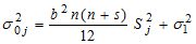 | (7) |
and  is the error variance, assumed equal to 1.Under the null hypothesis, the statistic
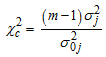 | (8) |
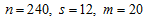
follows the chi-square distribution with  degrees of freedom, m is the number of observations in each column and
  is the number of columns. They stated that, the interval
 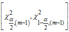 contains the statistic (8) with
  degree of confidence.The decision rule is to reject null hypothesis if calculated value of statistic lie outside the interval, otherwise do not reject H0.
2.1. Test for Constant Variance
Bartlett’s test allows the comparison of variance of two or more samples to determine whether they are drawn from populations with equal variance. It is appropriate for normally distributed data. To test the null hypothesis that the variances are equal, that is against the alternative
 and at least one variance is different from othersBartlett [1] has shown that, the statistic
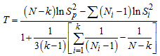 | (9) |
follows Chi-square distribution with (k – 1) degrees of freedom.Using the parameters of the Buys-Ballot table, 
 the statistic in (9) is then given as
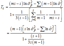 | (10) |
where  is the total number of observations,
  is the number of observations in each column and
  is length of the periodic interval.
3. Real Life Example
Real life example is based on monthly data on number of church marriages collected from Holy Cross Parish Owerri, Imo State, Nigeria, for the period 1997 to 2016 shown in Appendix A while the time plot is in Figure 3.1. The first step is to check whether the data admits the additive model. The modified Bartlett’s test statistic, given in (10) is used. The null hypothesis that the data admits additive model is rejected, if Tc is greater than the tabulated value, which for  level of significance and
  degrees of freedom equal to 19.7 or do not reject H0 otherwise.
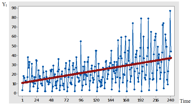 | Figure 3.1. Time plot for the actual series of number of church marriages between (1997-2016) |
Table 2. Column Variance
 of number of church marriages in a Buys-Ballot table of number of church marriages in a Buys-Ballot table
 |
| |
|
From Appendix A and Table 2 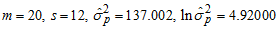 and
and 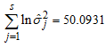 Hence,
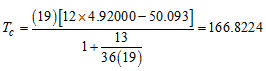 When compared with the critical value (19.7), Tc is greater, indicating that the data does not admit the additive model. Having confirmed that the data does not admit additive model, the choice now lies between mixed and multiplicative models. According to the proposed chi-square test by Nwogu, et al, [8], the null hypothesis that the data admits the mixed model is rejected, if the statistic defined in (8) lies outside the interval
 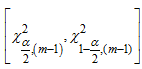 which for
  level of significance and
  degrees of freedom, equals (8.907, 32.85) or do not reject H0 otherwise.
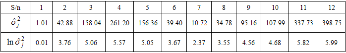
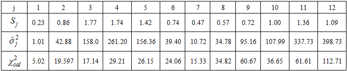
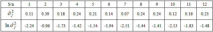
Table 3. Seasonal effects
 estimate of the column variance estimate of the column variance
 and Calculated Chi-square and Calculated Chi-square

 |
| |
|
From Appendix A and Table 3, 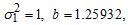
 Hence, from (7),
 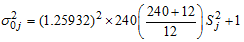 and the calculated values,
  given in Table 3 were obtained. When compared with the critical values (8.907 and 32.85), some of the calculated values lie outside the interval, indicating that the data does not admit mixed model. However, the result of the data evaluation shows that the data requires logarithm transformation to meet the constant variance and normality assumptions in the distribution. When the column variances of the logarithm transformed series given in Table 4 are subjected to test for constant variance, the calculated Bartlett’s test statistic (19.55) is less than the tabulated (19.7) at
  level of significance and
  degrees of freedom. This indicates that the variance is constant and the transformed series admits additive model. This confirms the need to evaluate data for possible transformation before applying the proposed test.
Table 4. The column variance
 of the transformed data in a Buys-Ballot table of the transformed data in a Buys-Ballot table
 |
| |
|
From Appendix B and Table 4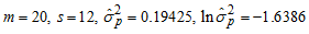 and
and 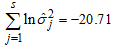 Hence,
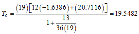
4. Concluding Remarks
This paper has discussed the Buys-Ballot modeling of church marriages in Imo State, Nigeria. The method adopted is Buys-Ballot procedure developed for choice of appropriate and choice of model among other uses, based on row, column and overall totals, averages and variances of the Buys-Ballot table. Result from calculated value of test statistic show that, the variance is constant and the transformed series admits additive model. This further confirms that the appropriate model of original data is multiplicative. There is indication that choice of model may be affected by violation of underlying assumptions, therefore, it is recommended that a study series should be evaluated for the assumptions of time series model before applying test for choice of model.
Appendix A
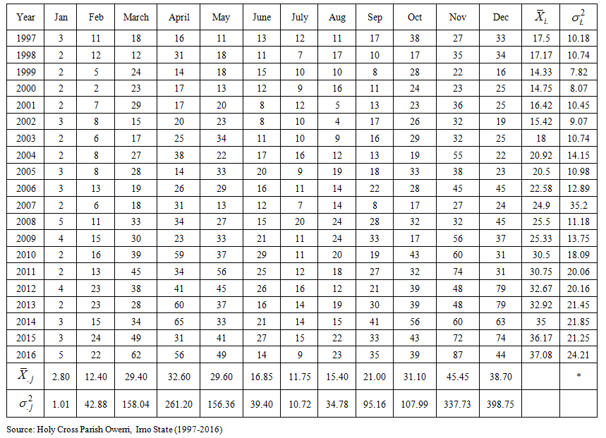 | Buys-Ballot table for the data on number of church marriages at Holy Cross Parish Owerri, Imo State (1997-2016) |
Appendix B
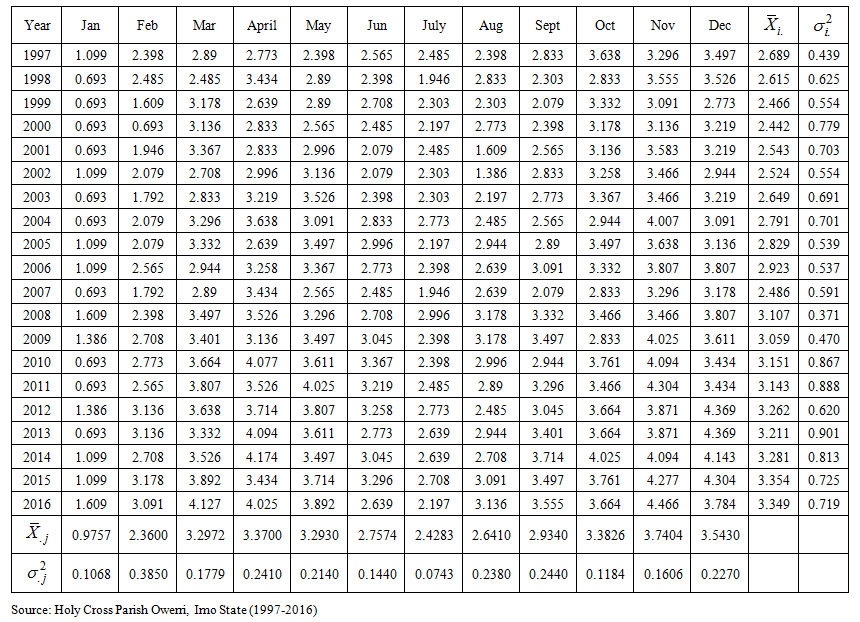 | Buys-Ballot table for the transformed data on number of church marriages at Holy Cross Parish Owerri, Imo State (1997-2016) |
References
| [1] | Bartlett, M. S. (1947). The use of transformations, Biometrika, 3, pp. 39-52. |
| [2] | Box, G. E. P., Jenkins, G. M., & Reinsel, G.C., (1994). Time Series Analysis: Forecasting and Control (3rd ed.). Englewood Cliffs N. J, Prentice-Hall. |
| [3] | Chatfield, C. (2004). The analysis of time Series: An introduction. Chapman and Hall, /CRC Press, Boca Raton. |
| [4] | Iwueze, I. S. and E. C. Nwogu (2004). Buys-Ballot estimates for time series decomposition, Global Journal of Mathematics, Vol. 3, No. 2, pp 83-98. |
| [5] | Iwueze, I.S., Nwogu, E.C., Ohakwe, J. & Ajaraogu. J.C (2011). Uses of the Buys – Ballot table in time series analysis. Applied Mathematics Journal 2, 633 –645. |
| [6] | Linde, P. (2005). Seasonal Adjustment, Statistics Denmark. www.dst.dk/median/konrover/13-forecasting-org/seasonal/001pdf. |
| [7] | Ljung, G. M. & Box, G. E. P. (1978). On a measure of lack of fit in time series models. Biometrika, 65, 297-303. |
| [8] | Nwogu, E.C, Iwueze, I.S. Dozie, K.C.N. & Mbachu, H.I (2019). Choice between mixed and multiplicative models in time series decomposition. International Journal of Statistics and Applications. 9(5), 153-159. |
| [9] | Oladugba, A.V., Ukaegbu, E.C., Udom, A.U., Madukaife, M.S., Ugah, T.E. & Sanni, S.S., (2014). Principles of Applied Statistic, University of Nigeria Press Limited. |

 Abstract
 Reference
 Full-Text PDF
 Full-text HTML