-
Paper Information
- Paper Submission
-
Journal Information
- About This Journal
- Editorial Board
- Current Issue
- Archive
- Author Guidelines
- Contact Us
American Journal of Mathematics and Statistics
p-ISSN: 2162-948X e-ISSN: 2162-8475
2020; 10(1): 10-19
doi:10.5923/j.ajms.20201001.02

Modelling and Forecasting Seasonal Behavior of Rainfall in Abuja, Nigeria; A SARIMA Approach
 Abstract
 Reference
 Full-Text PDF
 Full-text HTML
Samuel Olorunfemi Adams1, Muhammad Ardo Bamanga2
1Department of Statistics, University of Abuja, Abuja, Nigeria
2Department of Mathematical Sciences, Kaduna State University, Kaduna, Nigeria
Correspondence to: Samuel Olorunfemi Adams, Department of Statistics, University of Abuja, Abuja, Nigeria.
| Email: |  |
Copyright © 2020 The Author(s). Published by Scientific & Academic Publishing.
This work is licensed under the Creative Commons Attribution International License (CC BY).
http://creativecommons.org/licenses/by/4.0/

The need to have a quantitative means of modelling and predicting rainfall is very important for the purposes of Airplane movements, Agriculture, planning and policy formulation. The aim of this study is to propose a model of Seasonal Autoregressive Integrated Moving Average (SARIMA) model to model and forecast the monthly frequency of the rainfall in Abuja, Nigeria for the period 1996 to 2018. The data was obtained from Nigerian Meteorological Agency (NiMet) Abuja, Nigeria and the analysis was based on probability Seasonal time series modelling approach. The Plot of the original data shows that the time series is stationary and the Augmented Dickey-Fuller test did not suggest otherwise. The graph further displays evidence of seasonality and it was removed by seasonal differencing. The plots of the ACF and PACF show spikes at seasonal lags, the minimum Akaike information criterion (AIC) was 3618.5, Bayesian Information Criterion (BIC) was 3624.3, maximum Coefficient of Determination (R2) was 0.799 and all the parameters of the proposed SARIMA model were statistically significant at p < 0.05, suggesting SARIMA (0, 0, 2)(0, 1, 2)12 as the best for modeling and predicting the monthly rainfall in Abuja, Nigeria. The fitted model was used to make forecast for the next four proceeding years, the average predicted rainfall for the peak periods i.e. April, May, June, July, August and September for the years; 2019, 2020, 2021 and 2022 were; 335.5mm, 337.5mm, 339.3mm and 341.2mm respectively, this implies; a 3.5%, increase in rainfall from 2018 to 2019, 4.% increase in rainfall from 2018 to 2020, 4.7%, increase in rainfall from 2018 to 2021 and a 5.2%, increase in rainfall from 2018 to 2022. The results are useful for predicting the expected rainfall in Abuja in the next four years and also provide information that would be helpful for decision makers in formulating policies, planning and mitigating the problems of flooding in Abuja. Thus, the study recommends among others that Federal Government and minister of the federal capital territory, Abuja should commence the process of avoiding flood by building dikes, levees and provision of adequate drainage systems in the city.
Keywords: ACF, Seasonality, Stationarity, PACF, Rainfall, SARIMA
Cite this paper: Samuel Olorunfemi Adams, Muhammad Ardo Bamanga, Modelling and Forecasting Seasonal Behavior of Rainfall in Abuja, Nigeria; A SARIMA Approach, American Journal of Mathematics and Statistics, Vol. 10 No. 1, 2020, pp. 10-19. doi: 10.5923/j.ajms.20201001.02.
Article Outline
1. Introduction
- Rainfall is the total amount of separate water drops which fall to the earth from the clouds, having been formed by the condensation of water vapor in the atmosphere. Condensation of this water vapor is brought about by the rise of air considerable height above the earth’s surface, during a given time, rainfall is measure by an instrument call rain gauge. [1] defined rainfall intensity duration frequency relationships as graphical representations of the amount of water that falls within a given period of time. These graphs are used to determine when an area will be flooded, and when a certain rainfall rate or a specific volume of flow will reoccur in the future. According to [2], rainfall frequency analyses are used extensively in the design of systems to handle storm runoff, including roads, culverts and drainage systems. [3] States that “the precipitation frequency analysis problem is to compute the amount of precipitation y falling over a given area in a duration of x minutes with a given probability of occurrence in any given year.” For engineering design applications, it is necessary to specify the temporal distribution of rainfall for a given frequency, or return interval. According to [4], IDF or Depth-Duration-Frequency (DDF) curves “allow calculation of the average design rainfall intensity [or depth] for a given expedience probability over a range of durations” and is the result of the rainfall frequency analysis. IDF estimates are important statistical summaries of precipitation records used for hydrologic engineering design [5]. The rain in Nigeria is characterized by high intensity rainfall, high frequency of rain occurrence and the increased presence of large raindrops when compared with temperate climates [6]. In Southeastern Nigeria, IDF curves are not readily available. Also the number of years of data used to develop a few IDF curves for the region found in the literature were rather short, [7] and [8]. A lot of attention has been directed towards modelling and forecasting the amount of rainfall in various parts of Nigeria. For example: In Ikeja, Lagos state [9], [10], Sahel Region in Nigeria, [11], Bauchi, [12], climatic zones in Nigeria, [13], Akure, Ondo state [14], Osun State [15], [16], Ile-Ife, Osun State [17], Umuahia, Abia State [18], Ota, Ogun State [19], Ogbomosho, Oyo State [20], ilorin [21]. There are also vast studies on modelling and forecasting of the frequency of rainfall outside Nigeria. In Bangladesh [22], Iran [23], Jordan [24], Golastan Province [25], East Africa [26] and Turkey [27].The aim of this study is to propose a Seasonal Autoregressive Integrated Moving Average (SARIMA) model for modelling and forecasting the monthly rainfall in Abuja for the period 1996 – 2018. Following the introduction, theoretical framework is presented in section 2, review of related literatures in section 3. Section 4 presents the materials and methods of the study. Section 5 presents results and discussions and finally, conclusions and recommendations are presented in section 6.
2. Theoretical Framework
2.1. Study Area
- Abuja is the capital city of Nigeria located in the centre of the country within the Federal Capital Territory (FCT)[28]. It is a planned city and was built mainly in the 1980s, replacing the country's most populous city of Lagos as the capital on 12th December 1991. [29] Abuja's geography is defined by Aso Rock, a 400-metre (1,300 ft) monolith left by water erosion. The Presidential Complex, National Assembly, Supreme Court and much of the city extend to the south of the rock. Zuma Rock, a 792-metre (2,598 ft) monolith, lies north of the city on the expressway to Kaduna. At the 2006 census, the city of Abuja had a population of 776,298, [30] making it one of the ten most populous cities in Nigeria. According to the United Nations, Abuja grew by 139.7% between 2000 and 2010, making it the fastest growing city in the world, [31]. As of 2015, the city is experiencing an annual growth of at least 35%, retaining its position as the fastest-growing city on the African continent and one of the fastest-growing in the world, [32]. As at 2016, the metropolitan area of Abuja is estimated at eight million persons, placing it behind only Lagos, as the most populous metro area in Nigeria, [33].Abuja experiences three weather conditions annually, this includes a warm, humid rainy season and an extremely hot dry season. In between these seasons, there is a short period of harmattan accompanied by the North East Trade Wind, with the main feature of dust haze, intensified coldness and dryness. The rainy season begins from April and ends in October, when daytime temperatures reach 28-30 degrees and night time lows range around 22-23 degrees. In the dry season, daytime temperatures can soar to 40 degrees and night time temperatures can drop to 12 degrees, resulting in chilly evenings. Even the chilliest nights can be followed by daytime temperatures well above 30 degrees. The high altitudes and rolling terrain of the FCT act as moderating influence on the weather of the territory. Rainfall in the FCT reflects the territory's location on the windward side of the Jos Plateau and the zone of rising air masses. The annual total rainfall is in the region of 1100 mm to 1600 mm.
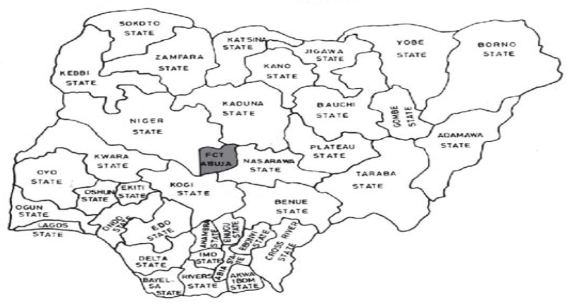 | Figure 1. Map of Nigeria showing Abuja, Federal Capital Territory |
3. Review of Empirical Literature
- Rainfall characteristics in Nigeria have been examined for dominant trend notably by [34] and [35]. They showed that there has been a progressive early retreat of rainfall over the whole country, and consistent with this pattern, they reported a significant decline of rainfall frequency in September and October which, respectively coincide with the end of the rainy season in the northern and central parts of the country. The pattern of rainfall in northern Nigeria is highly variable in spatial and temporal dimensions with inter-annual variability of between 15 and 20% [36]. As a result of the large inter-annual variability of rainfall, it often results in climate hazards, especially floods and severe and droughts with their devastating effects on food production and associated calamities and sufferings [37-39]. Rainfall is one of the key climatic resources of Akwa-Ibom State. Crops and animals derived their water resources largely from rainfall. It is considered as the main determinant of the types of crops that can be grown in the area and also the period of cultivation of such crops and the farming systems that can be practiced. [40] upheld and modelled the frequency of monthly rainfall in Umuahia the Abia State capital in NIgeria with SARIMA (0, 0, 0)(0, 1, 1)12 model after favourably competing with SARIMA (0, 0, 0)(1, 1, 1)12 model. However, the model was found satisfactory in forecasting the future Frequency of monthly rainfall in Umuahia and was therefore recommended for this task. Also, [40] found the parsimonious SARIMA (1, 2, 1)(0, 0, 1)12 model after favourably competing with SARIMA (11, 2, 1)(0, 0, 1)12 model as the best fit to the Nigeria's average rainfall using 19 years monthly data from January, 1996 to December, 2013. The SARIMA (1, 2, 1)(0, 0, 1)12 model satisfactorily forecast the future Nigeria's rainfall amount. [40] analyzed the monthly rainfall obtained from National Root Crops Research Institute Umudike in Nigeria from 1996 to 2011 based on probability time series modelling approach. The Plot of the original data shows that the time series is stationary and the Augmented Dickey-Fuller test did not suggest otherwise. The graph further displays evidence of seasonality and it was removed by seasonal differencing. The plots of the ACF and PACF show spikes at seasonal lags respectively, suggesting SARIMA (0,0,0) (1,1,1)12. Though the diagnostic check on the model favoured the fitted model, the Auto Regressive parameter was found to be statistically insignificant and this led to a reduced SARIMA (0, 0, 0) (0, 1, 1)12 model that best fit the data and was used to make forecast. Comparison of the actual/observed frequency from July to December 2011 was done with their corresponding forecast values and a t-test of significance showed no significant difference. [10] identified and established the adequacy of the Seasonal ARIMA (5,1,0)(0,1,1)12 for modelling and forecasting the amount of monthly rainfall in Port-Harcourt, Nigeria. [41] examined the rainfall availability to crop yield in south-south region of Nigeria, the study showed a gradual decline in rainfall trend as from the coastal south to the northern part of the state. Even though the northern part of the state tends to indicate abysmal increase in annual rainfall trend, a decline in annual rainfall of 58% and 65% of the total period was observed for the coastal south (Eket) and the central part (Uyo) of the state respectively. This decline was more pronounced in the months of March, July and September. Generally, the observed decline in rainfall trend may be due to the migration pattern of the region of Inter-Tropical Discontinuity (ITD) – a region of convergence of the trade wind and the monsoonal air flow. [11] used monthly rainfall data of thirty six (1981-2017) years for some stations in the Sahel region of the country (they include, Katsina Zamfara, Maiduguri, Sokoto, Yobe states) obtained from the archive of the Nigerian meteorological Agency, NiMet. The data were then subdivided into segments (1981-2014, 1981-2015 and 1981-2016) in order to train ARIMA models for the states in the region. The models were subsequently validated and used to forecast monthly rainfall for the aforementioned states. Statistical t-test were then employed to ascertain differences between the forecast and actual rainfall data for 2015, 2016 and 2017. The results of the t-test carried out at the 1 and 5% level of significance indicated that there was no significant difference between the forecast and actual rainfall. Accordingly it is recommended that the developed arima models, which of course differ from one state to the other, could be adopted and used to generate forecast of monthly rainfall for year 2018. Although statistical t-test indicated no difference between forecast generated from the model and the corresponding actual data, the models appeared to have performed better over Gusau (in 2016 and 2017), Katsina (2016 and 2017), Potiskum (in 2016) and Sokoto. [14] worked on statistical analysis of rainfall trend in Akure, Ondo state, Nigeria. Descriptive statistics (mean and standard deviation) and inferential statistics (time series and correlation analysis) were in their analysis. The results from time series analysis showed that rainfall fluctuated in an upward trend through the period of study. The predicted rainfall for 2016-2045 indicated a positive trend of (+0.274), meaning that rainfall will increase in intensity, number of raining-days and duration. The study equally revealed a significant increase in rainfall trend for Akure between 1966 and 2015. [15] proposed SARIMA model for Osun State monthly rainfall data and the analysis was based on probability time series, the plots of the ACF and PACF show spikes at seasonal lags respectively, suggesting SARIMA (1, 0, 1) (2, 1, 1). Though the diagnostic check on the model favoured the fitted model, the Auto Regressive parameter was found to be statistically insignificant and this led to a reduced SARIMA (1, 0, 1) (1, 1, 1) model that best fit the data and was used to make forecast. [21] examined the stochastic characteristics of the Ilorin monthly rainfall in Nigeria using four different modeling techniques (Decomposition, Square root transformation-deseasonalisation, Composite and Periodic. Autoregressive) where they compared the results from the various methods employed. Outside Nigeria, there are also vast studies on modelling and forecast of rainfall. In Bangladesh, [22] used Box-Jenkins methodology [42] to build seasonal ARIMA model for monthly rainfall and temperature data taken for Bangladesh, for the period between 1981-2010. In their work, ARIMA (0, 0, 1) (0, 1, 1) 12 model was found adequate and the model is used for forecasting the monthly rainfall and temperature. In Iran [23], use time series method to model weather parameter in Iran and recommended ARIMA (0, 0, 1)(1, 1, 1)12 as the best fit for monthly rainfall data and ARIMA (2, 1, 0)(2, 1, 0)12 for monthly average temperature for the region. [24] dealt with the statistical analysis of the rainfall measurements for three meteorological stations in Jordan: Amman Airport (central Jordan), Irbid (northern Jordan) and Mafraq (eastern Jordan). Normal statistical and power spectrum analyses as well as ARIMA model were performed on the long-term annual rainfall measurements at the three stations. The result shows that possible periodicities of the order of 2.3-3.45, 2.5-3.4 and 2.44-4.1 years for Amman, Irbid and Mafraq stations, respectively, were obtained. A time series model for each station was adjusted, processed, diagnostically checked and lastly an ARIMA model for each station is established with a 95% confidence interval and the model was used to forecast 5 years annual rainfall values for Amman, Irbid and Mafraq meteorological stations. [25] analyzed the precipitation forecast using SARIMA model and found the seasonality measure in SARIMA to be highly useful in measuring precipitation. [26] used time series methods based on ARIMA and Spectral analysis of a real annual rainfall of two homogenous region in East Africa and recommended ARMA (3,1) as the best fit for areal indices of relative wetness\dryness and dominant quasi-periodic fluctuation around 2.2-2.8 years, 3-3.7 years, 5-6 years and 10-13 years. [27] examined the temporal characteristics of rainfall variability in Africa using departure series for 84 regions of the continent and five larger-scale zones. The forms of non-randomness which are investigated include linear trends, persistence and quasi-periodic fluctuations. No long-term trends in African rainfall are evident. In some sectors, most notably along the Benguela coast and equatorial Africa, rainfall anomalies tend to persist over several months and interseasonal correlations are also high. Spectral analysis revealed significant quasi-periodicities clustered in four bands at 2.2–2.4, 2.6–2.8, 3.3–3.8 and 5.0–6.3 years. [43] used Autoregressive Integrated Moving Average (ARIMA) and Seasonal Autoregressive Integrated Moving Average (SARIMA) models to analyzed the accuracy and trend of time series of the monthly rainfall and predicated for the succeeding year. The results showed that the model fitted into the data well and the stochastic seasonal fluctuation was successfully modeled. [44]modeled and forecasted the daily air temperature and precipitation time series recorded between January 1, 1980 and December 31, 2010 in four European sites (Jokioinen, Dikopshof, Lleida and Lublin) from different climatic zones. The forecasting used the methods of the Box-Jenkins and Holt-Winters seasonal Auto Regressive integrated moving-average, the Autoregressive Integrated moving-average with external regressors in the form of Fourier terms and the time series regression, including trend and seasonality components methodology with R software. It was demonstrated that obtained models are able to capture the dynamics of the time series data and produced sensible forecasts. Dabral and Murry (2017) [45] used Seasonal Auto Regressive Integrative Moving Average models (SARIMA) to develop monthly, weekly and daily monsoon rainfall time series. Using Box-Cox transformation and subsequently differencing, monthly, weekly and daily monsoon rainfall time series were made stationary. The best SARIMA models were selected based on the autocorrelation function (ACF) and partial autocorrelation function (PACF), and the minimum values of Akaike Information Criterion (AIC) and Schwarz Bayseian Information (SBC). As per Ljung-Box Q statistics, residuals random in nature and there was no need for further modelling. Performance and validation of the SARIMA models were evaluated based on various statistical measures. The mean and standard deviation of the predicted data were found close to the observed data. Nash-Sutcliffe coefficient also indicated a high degree of model fitness to the observed data. Forecasting of monthly, weekly, daily monsoon time series for 14 years, i.e., from 2014 to 2027 was done using the developed SARIMA model. Rainfall was minimal in January, February, March and December over the selected stations in northern, Nigeria but increased progressively in strength and amount in the months of June, August and September over the stations in South west, and June and September over the stations in South-south, Nigeria. The highest rainfall of 230 mm was recorded in September over Warri and the lowest rainfall of 52 mm was recorded in August over Maiduguri. Furthermore, efforts have been made by [46] and [47] to obtain 1-minute rain rate map, and rain rate estimation respectively for Nigeria, using Rice-Holmberg (R-H) model.
4. Material and Methods
4.1. Data Source
- The data used in this study is a secondary data of the monthly rainfall (mm), it was obtained from Nigeria Meteorological Agency (NiMet), Abuja station, Nigeria. The data spanned between the periods 1996 to 2018 (twenty-two years).
4.2. Seasonal Autoregressive Integrated Moving Average (SARIMA) Model
- Seasonal Autoregressive Integrated Moving Average (SARIMA) model is an algebraic statement that describes how a time series is statistically related to its own past. The seasonal ARIMA model incorporates both non-seasonal and seasonal factors in a multiplicative model given as;
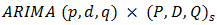 | (1) |
 | (2) |
 | (3) |
 | (4) |
 | (5) |
 | (6) |
 , if seasonality is on the AR portion, and
 , if seasonality is on the MA portion, where
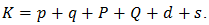
  Identification of the ARIMA model: Three goodness-of fit statistics that are most commonly used for the model selection are; Coefficient of determination (R2), Akaike Information Criterion (AIC) and Schwarz Bayesian Information Criterion (BIC) [41-42]. The AIC and BIC are determined based on a likelihood function. The AIC and BIC are calculated using the formulas below:
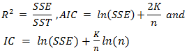 | (7) |
5. Results and Discussion
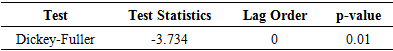
- From the plots in Figure 2 it could be seen that the time series plot displays a wave like pattern an evidence of seasonality and no trend is observed which implies that the time series is stationary. The sinusoidal or periodic pattern in the ACF plot is again suggesting that the series has a strong seasonal effect also, the PACF plot is neither suggesting otherwise. In order to verify the stationarity claim of the visual displays an Augmented Dickey-Fuller test [43] was performed with hypothesis;H0: The rainfall data is unit root non stationary andH1: The rainfall data is stationary.
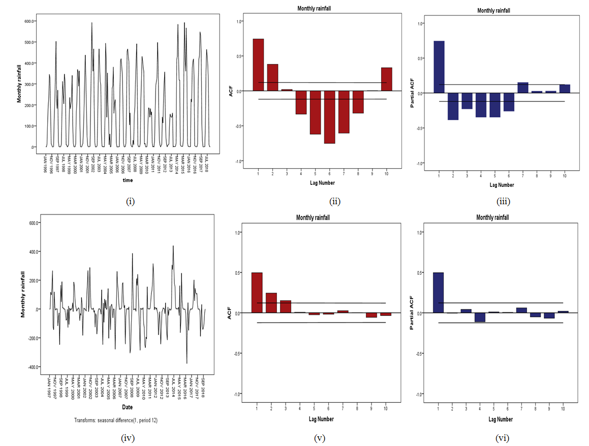 | Figure 2. (i) Time Series Plot of the Original data, (ii) & (iii)-ACF and PACF Plots Respectively of the Original data, (iv) Time Series Plot of the seasonal Differenced s, (v) & (vi)-ACF and PACF Plots Respectively of the Differenced Logged-data |
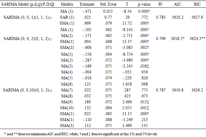
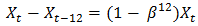 and the data is re-examined visually. All the plots in Figure 3 shows that the first seasonally differenced rain fall series in now well behaved. The ACF of the original un-difference series show a significant positive cut-off at lag 1, 2 and 10, suggesting MA (q) = 1, 2,10, while the PACF of the original non-difference series show a significant positive cut-off at lag 1, suggesting AR (p) = 1. The pronounced spikes at the first, second and third seasonal lags of the ACF suggest, MA (Q) = 1,2,3 and the spike at the first seasonal lag of PACF plot suggests, AR (P) =1 with first seasonal difference (D) = 1, Therefore, proposed Seasonal ARIMA are; SARIMA (0, 0, 1)(1, 1, 1)12, SARIMA (0, 0, 2)(0, 1, 2)12 and SARIMA (0, 0,10)(0, 1, 3)12. The suggested SARIMA models were compared based on the following criteria; coefficient of the proposed models, t-statistics, p-values, standard errors, R2, AIC and BIC respectively. The SARIMA (0, 0, 2)(0, 1, 2)12 clearly proved to be the appropriate model with minimum Akaike information criterion (AIC) of 3618.5, Bayesian Information Criterion (BIC) of 3624.3 and maximum Coefficient of Determination (R2) of 0.799 and all the parameters of the fitted SARIMA (0, 0, 2)(0,1,2) model in Table 2 are statistically significant at p < 0.05. The diagnostic check of the fitted SARIMA (0, 0, 2)(0, 1, 2) model is presented in Figure 3(i-ii), it shows the overall adequacy of the fitted model, where the standardized residual plot shows that the residuals are standard normal distributed on N (0, 1), the ACF and PACF plot also shows that the residuals are uncorrelated at the lags. Fig. 3 shows the time series of the standardized residuals. The plot depicts no pattern, a clear indication that the standardized residuals behaves like a typical white noise process as required. The goodness of fit of the two tentatively identified models would be judged on the basis of their information criterion statistics (BIC) and Akaike Information Criterion (AIC) [18].
|
|
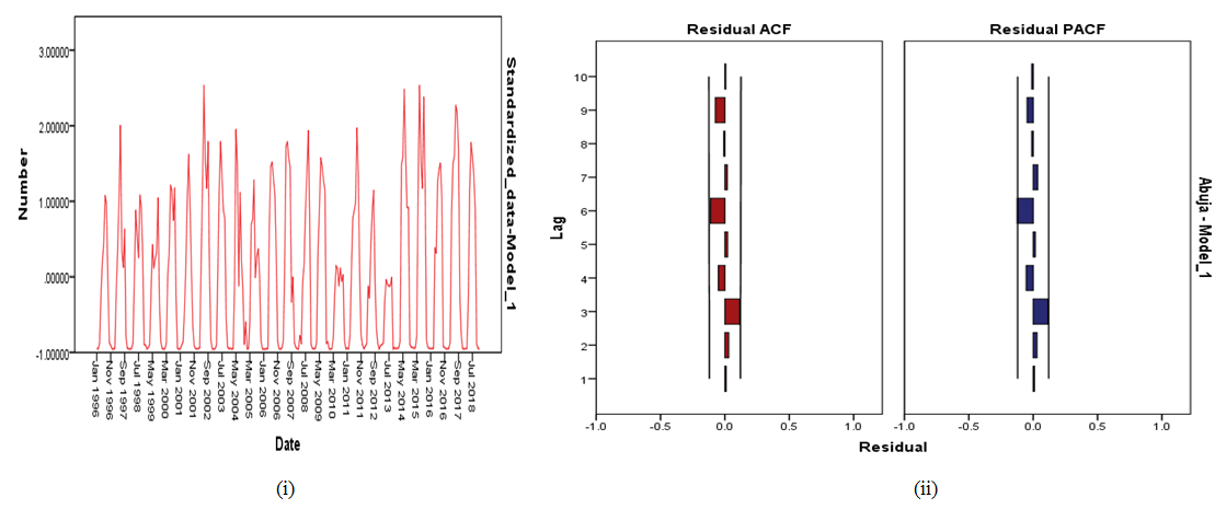 | Figure 3. (i) The Standardized Residual Plot of the Fitted SARIMA(0,0,2)(0, 1, 2) and (ii) ACF and PACF Plots Respectively of the standardized residual of the fitted SARIMA (0,0,2)(0,1,2) Model |
5.1. Forecasting with the Fitted Models
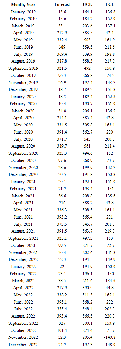
- The selected model was then used to describe and forecast the time series observations for the next three years (January 2019 – December 2022) as presented in table 3. Using SARIMA (0, 0, 2)(0, 1, 2) Model, the average monthly rainfall in 2018 was 173.4mm, while the average predicted monthly rainfall for year 2019, 2020, 2021 and 2022 were; 184.8mm, 186.9mm, 188.8mm and 190.7mm respectively, this implies that, there will be a 6.6%, increase in rainfall from 2018 to 2019, 7.8% increase in rainfall from 2018 to 2020, 8.9%, increase in rainfall from 2018 to 2021 and a 10.0%, increase in rainfall from 2018 to 2022. Fig. (4) Shows the past (red lines) and forecast (blue lines) time series of the original monthly rainfall data in Abuja, with the fitted SARIMA model while the dashed lines in both plots indicate the 95% confidence intervals.
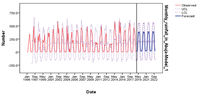 | Figure 4. Forecast of the Monthly rainfall in Abuja and its 95% confidence interval |
|
 Vs
Vs
|

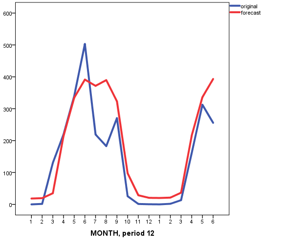 | Figure 5. Time series of monthly rainfall forecast( red line) and observed monthly (blue line) rainfall in Abuja |
6. Conclusions and Recommendations
- In this study, the frequency of monthly rainfall from 1996 to 2018 obtained from Nigeria Meteorological Agency (NiMet), Abuja station, Nigeria. The data spanned between the period 1996 to 2018 (twenty-two years). The data was analysed using probability time series modelling approach. The Plot of the original data shows that the time series is stationary and has evidence of seasonality. The Augmented Dickey-Fuller test confirmed the stationarity claim. Seasonal differencing was done to remove the seasonal effect. SARIMA modelling of the data was upheld after duly following the conventional three steps of identification, estimation and diagnostic checking procedures established by Box and Jenkins. The SARIMA (0, 0, 2)(0, 1, 2)12 clearly proved to be the appropriate model with minimum Akaike information criterion (AIC) of 3618.5, Bayesian Information Criterion (BIC) of 3624.3 and maximum Coefficient of Determination (R2) of 0.799 and all the parameters of the fitted SARIMA (0, 0, 2)(0,1,2) model were statistically significant was used to make forecast. The average rainfall in the four months peak periods in 2018 was 324.2mm, while the average predicted rainfall for the peak periods i.e. April, May, June, July, August and September for the years; 2019, 2020, 2021 and 2022 were; 335.5mm, 337.5mm, 339.3mm and 341.2mm respectively, this implies that, there will be a 3.5%, increase in rainfall from 2018 to 2019, 4.1% increase in rainfall from 2018 to 2020, 4.7%, increase in rainfall from 2018 to 2021 and a 5.2%, increase in rainfall from 2018 to 2022. Comparison of the observed and forecasted frequency of some selected values analyzed with a t-test showed no significant difference.The results are useful for predicting the expected rainfall in Abuja in the next four years and also provide information that would be helpful for decision makers in formulating policies to mitigate the problems of flooding in Abuja. The percentage increments in the predicted rainfall frequency in Abuja, Nigeria is an indication of flood, it is therefore recommended that the Federal Government and minister of the federal capital territory, Abuja should commence the process of avoiding flood by building dikes, levees and provision of adequate drainage systems.