Akintunde Mutairu O.1, Chigozie Kelechi A.2, Agunloye Oluokun K.3, Oyekunle Janet O.1, Agbona Anthony A.1, Kgosi Phazamile M.4
1Department of Statistics, Federal Polytechnic, Ede, Osun State, Nigeria
2Michael Okpara University of Agriculture, Umudike, Abia State, Nigeria
3Department of Mathematics, Faculty of Science Obafemi Awolowo University, Ile-Ife, Osun State, Nigeria
4Department of Statistics, Faculty of Social Sciences University of Botswana,Gaborone, Botswana
Correspondence to: Akintunde Mutairu O., Department of Statistics, Federal Polytechnic, Ede, Osun State, Nigeria.
| Email: |  |
Copyright © 2019 The Author(s). Published by Scientific & Academic Publishing.
This work is licensed under the Creative Commons Attribution International License (CC BY).
http://creativecommons.org/licenses/by/4.0/

Abstract
The paper provides an understanding about the theoretical and empirical illustration of working of various classes of ARCH family models used in the study. It equally exploits the potential benefits derivable from using this family type models. It dwells heavily into the best time series model among autoregressive moving average (ARMA), Autoregressive conditional heteroscedasticity (ARCH), Generalized Autoregressive conditional heteroscedasticity (GARCH), Integrated Generalized Autoregressive conditional heteroscedasticity (IGARCH), Threshold Generalized Autoregressive conditional heteroscedasticity (TGARCH) and Exponential Generalized Autoregressive conditional heteroscedasticity (EGARCH) models, and determined the models which actually give the best forecast performance. Mathematical background of all these models were set up and promptly illustrated using monthly data of number of patients admitted for malaria at Ladoke Akintola teaching hospital, Osogbo. It covers the period of five years (2012 January to December, 2016), obtained from the hospital record of LAUTECH, Osogbo. Stationarity tests (graph, unit root and correlgram) were conducted before proceeding to parameter estimations. The grid search using Akaike information criteria (AIC) and Performance measures indices were used to determine the best model. So also, performance measure indices were cross tabulated with the models. In all, out of seven performance measure indices used, EGARCH (1,1) Model is best in the six of the indices. From these results EGARCH (1,1) is recommended for would be investors, forecasters and other categories of users.
Keywords:
ARMA, ARCH, GARCH, IGARCH, EGARCH and TGARCH
Cite this paper: Akintunde Mutairu O., Chigozie Kelechi A., Agunloye Oluokun K., Oyekunle Janet O., Agbona Anthony A., Kgosi Phazamile M., Evaluating the Forecast Performance of Autoregressive Conditional Heteroscedasticity (ARCH) Family Models, American Journal of Mathematics and Statistics, Vol. 9 No. 6, 2019, pp. 221-227. doi: 10.5923/j.ajms.20190906.03.
1. Introduction
In conventional time series models, the major assumption behind the least square regression is homoscedasticity i.e constant variance. If this condition is violated, the estimates will still be unbiased but they will not be minimum variance estimates. The standard error and confidence intervals calculated in this case become too narrow, giving a false sense of precision. But many financial time series such as exchange rate, stock market indices, market returns, inflation rate and so on exhibit periods of unusual large volatility, followed by periods of relative tranquility (time series exhibits clustering of large and small disturbances). Such situations suggest a form of heteroscedasticity in which the variance of the disturbance depends on the size of preceding disturbance and hence the conditional variance is non-constant over the sample period. The ARCH models have the ability to capture all the above characteristics in financial market variables. ARCH and related models can handle this by modeling volatility itself in the model and thereby correcting the deficiencies of least squares model.Forecasting has attracted the interest of many academicians, investors and policy makers. Hence various models ranging from simplest models such as random walk to the more complex conditional heteroskedastic models of the GARCH family have been used to forecast financial series. [1] is the first one who uses GARCH model to forecast, he shows that GARCH produces better forecast than most of the other forecasting methods such as Random Walk (RW), Historical Mean (HM), Moving Average (MA) and Exponential Smoothing (ES) when applied to monthly US stock market data. In addition, [4] and [13] found that Threshold GARCH outperforms ARCH, GARCH, and Exponential GARCH on monthly US stock market data. On the other hand, [6] evaluate the forecasting accuracy of simple models such as Random Walk, Moving Average, Exponential Smoothing and Regression Models on UK stock market data and they conclude that Exponential Smoothing and Regression Models provide the best forecast. [2] investigate the forecasting performance of both ARCH-type models and non-ARCH models applied to 14 different countries. [11] use Moving Average, Historical Mean, Random Walk, GARCH, GJR-GARCH, EGARCH and APARCH to forecast volatility of two Chinese Stock Market indices; Shanghai and Shenzhen. Among GARCH models, GJR-GARCH and EGARCH outperforms other ARCH models for Shenzhen stock market. [9] employed Random Walk, GARCH(1,1), TGARCH(1,1) and EGARCH(1,1) to forecast Ghana Stock Exchange. GARCH(1,1) provides the best forecast according to three different criteria out of four. This paper therefore examines or evaluates the forecast performance of ARCH family models to number of patients admitted for malaria at Ladoke Akintola teaching hospital, Osogbo. The recent development global wise therefore requires the use of quantitative models that will have the ability to inform the players in all sectors the implication of the risks taking in one side and the returns on the other side.
2. Mathematical Specifications
2.1. Autoregressive Moving average (ARMA)
 Autoregressive moving average with orders
  model in a discrete time linear equation with noise of the form
 | (1) |
Or more explicitly as  | (2) |
We may incorporate a none zero average in the model. If we want that  has average of
  , the natural procedure is to have zero average solution
  of
of | (3) |
and take  have solution of
 | (4) |
With 
2.2. Autoregressive Conditional Heteroscedasticity (ARCH) Model
Suppose  are the time series observations (exchange rates, stock values and so on) and let
 be the set of
  up to time
  , including
  for
for  ≤ 0. As defined by [7], the process
  is an Autoregressive Conditional Heteroscedasticity process of order
  , if:
, if:  , with
 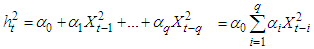 | (5) |
Where  ,
,  and
and  for
for  . The conditions
  and
and  are needed to guarantee that the conditional variance
  .
.
2.3. Generalized Autoregressive Conditional Heteroscedasticity (GARCH) Models
The Generalized Autoregressive conditional heteroscedasticity models were propounded by [7] and [3]. They were the first researchers to propose a stationary non-linear model for  , which he termed ARCH (Autoregressive conditional heteroscedaticity); this means that the conditional variance of
  evolves according to an auto regressive type process. [3] and [12] independently generalized Engle’s model to make it more realistic; the generalization was called “GARCH”. GARCH is probably the most commonly used financial time series model and has inspired dozens of more sophisticated models. The commonly used financial time series model is GARCH and so many sophisticated models were built from it.Definition: The
  model is defined by:
 | (6) |
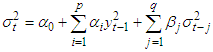 | (7) |
where  and the innovation sequence
  is independent and identically distributed with
  .
.
2.4. The Exponential Generalized Autoregressive Conditional Heteroscedasticity (p, q) Model
GARCH models, assume that only the magnitude and not the positivity or negativity of unanticipated excess returns determines features of  . If the distribution of
  is symmetric, the change in variance is conditionally uncorrelated. The Exponential
  model put forward by [10] is as follows
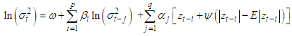 | (8) |
 given that
  , where the parameters
  are not restricted to be non-negative.
2.5. The Integrated Generalized Autoregressive Conditional Heteroscedasticity (p, q) Model
The  process characterized by the first two conditional moments:
 | (9) |
where  and
and  for all
  and the polynomial
  has
has  unit root(s) and
  outside the unit circle is said to bei. Integrated in variance of order
  ii. Integrated in variance of order
  with
with  The Integrated
  models, both with or without trend, are therefore part of a wider class of models with a property called "persistent variance" in which the current information remains important for the forecasts of the conditional variances for all horizons.So, we have
  models when necessary condition
2.6. Threshold Generalized Autoregressive Conditional Heteroscedasticity (TGARCH) OR GJR-GARCH
[8] (1994) proposed TGARCH process for asymmetric volatility structure.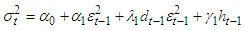 | (10) |
where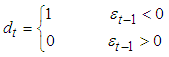 | (11) |
Where  , the negative shock will have larger effect on volatility.
2.7. Performance Measure Indices
i. Mean square error (MSE)The MSE serves to aggregate the magnitudes of the errors in predictions for various times into a single measure of predictive power. It is one of the commonly used error index statistics [5]. Although it is commonly accepted that the lower the MSE the better the model performance. MSE is given as: 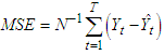 | (12) |
ii. Mean Absolute error (MAE)The absolute error is the absolute value of the difference between the forecasted value and the actual value. MAE tells us how big the size of an error we can expect from the forecast on average. This is mathematically given as: 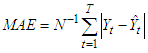 | (13) |
iii. Mean absolute precision error (MAPE)MAPE has indispensable statistical properties in that it makes use of all observations and has the smallest variability from sample to sample. It is also useful for purposes of reporting because it is expressed in generic percentage terms that will be understandable to a wide range of users and very simple to calculate and easy to understand, which attests to its popularity. It is given as: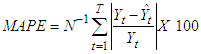 | (14) |
iv. Theil’s U inequality coefficientA more useful measure to evaluate the predictive accuracy of a model is Theil’s U inequality coefficient, which measures the root mean square error in relative terms, and is defined as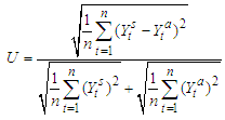 | (15) |
The denominator imposes an upper bound to the U coefficient, which is bounded above by 1 and bounded below by 0, that is, 0 ≤ U ≤ 1. This is particularly useful since it gives a threshold to evaluate the accuracy of a model and not only compare it to other models. The closer to 0 the coefficient is, the more accurate the model is, while a coefficient equal to 1 indicates that the forecast performance of the model is as bad as it could be. The U coefficient can be decomposed into three proportions that provide useful additional information on the performance of the model.Bias, 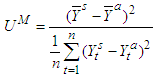 | (15a) |
Variance, 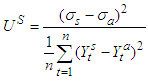 | (15b) |
Covariance,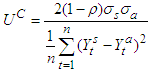 | (15c) |
The bias proportion measures the systematic error of the forecast; it gathers the share of the simulation error that comes from bias, that is, the difference between the averages of the forecasted series and the actual series. The variance proportion is intended to provide a measure of how well our forecast replicates the volatility of the actual series. The covariance proportion offers a measure of the unsystematic error in the forecast.
3. Data Analysis and Discussion of Results
3.1. Descriptive Statistics
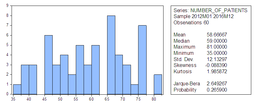 | Figure 1. Descriptive Statistics |
Figure 1 above revealed that the standard deviation is high which indicates high degree of fluctuations in number of patients data used; there is evidence of skewness with negative sign indicating that the data used is non-symmetric. From the histogram, the number of patients’ data is non-leptokurtic as its large kurtosis value is smaller compare to the mean. Jarque-Bera test with p-value less than zero shows that the data is non-normal so that the hypothesis of normality is rejected. From here the study proceeded to determination of stationarity of data used for the study before embarking on the analysis of the data.For any study to be valid in time series there is the need to verify the stationarity of the series involve before the analysis. Three important methods of checking stationarity of time series were used in this study; they are graphical, unit root and correlogram.
3.2. Graphical Method
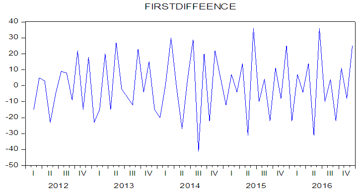
Figures 2 and 3 show the time plots for the data. The original data (figure 2) shows that the data is not stationary i.e fluctuating as it gives not too high coefficient of determination  of 0.588. More so, at the first difference, the data seems to be stationary as it gives a coefficient of determination of 0.864, the mean of the series is more stable at this level.
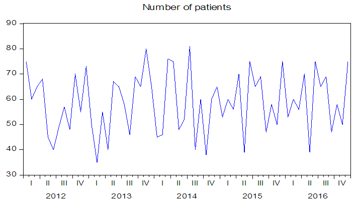 | Figure 2. Original data |
 | Figure 3. Differenced data |
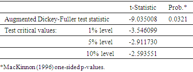
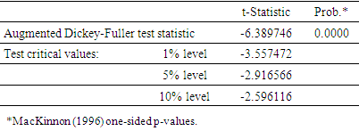
3.3. Unit Root
Table 1. Unit Root (Level)
 |
| |
|
Table 2. Unit Root First Difference
 |
| |
|
At level the probability value of the ADF is lesser than 5% i.e. prob. = 0.0000 < 0.05, but the test an only account for 58.8% fitness and cannot be accepted for being stationary while at first difference, value of the ADF is lesser than 5% i.e. prob. = 0.0000 < 0.05 and gives an account of 86.4% which is assumed to be a good fit, hence suggesting that the data is stationary.
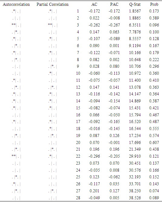
3.4. Correlogram
Table 3. Correlogram (Level)
 |
| |
|
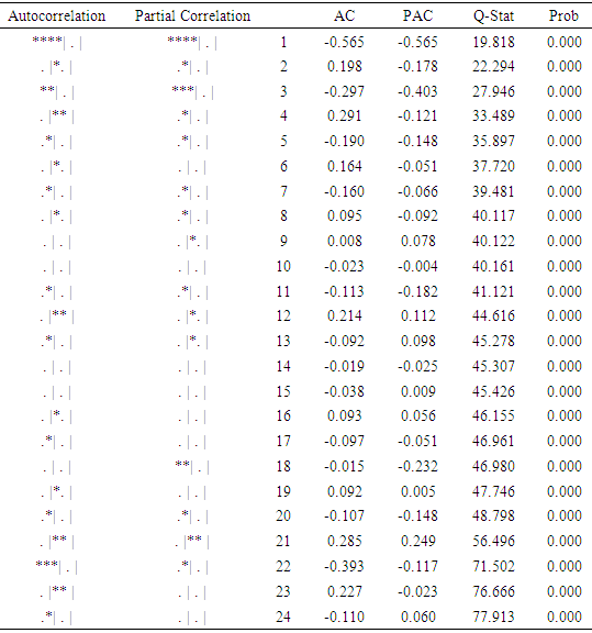
Table 4. Correlogram (First Difference)
 |
| |
|
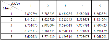
Interpretation: The correlogram of the series are given in tables 3 and 4. Table 3 Show the correlogram of the original data with autocorrelation coefficient that starts with a low value of 0.173 and declines very slowly towards zero which prove that the series is non-stationary. Furthermore, table 4 shows no trend in number of patients admitted data, hence suggesting that the infant mortality series is stationary.GRID SEARCHTable 5. Grid Search Table (Table 5)
 |
| |
|
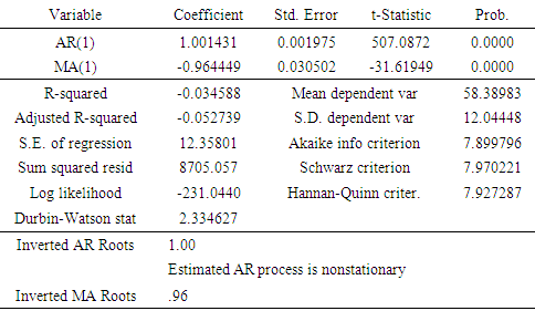
Interpretation:In table 5 above, both processes demonstrate correlation residuals. Among the different models applied to the data, GARCH(1,1) appears to be relatively better fit on the basis of Akaike Information Criterion. The results of GARCH (1,1) are shown in table 6 below: Table 6
 |
| |
|
3.5. Parameter Estimates
The models earlier listed were subjected to parameter estimation, from the analysis the following details relating to parameter estimates of all the models used. They are as listed below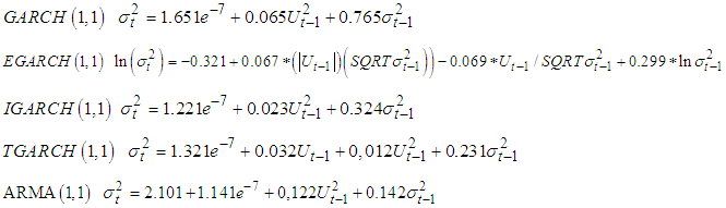
3.6. Comparison of Forecast Performance
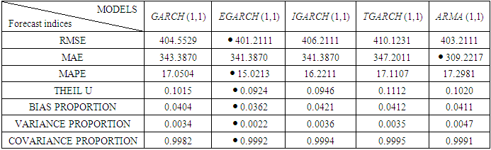
Various forecast measuring indices were cross tabulated with the models used in the study. The forecast measurement indices used are Root mean square error (RMSE), Mean absolute error (MAE), Mean absolute precision error (MAPE), Theil U-inequalities, Bias proportion, Variance proportion and Covariance proportion. The table of comparison as obtained from the analysis were extracted and shown in the table 7 as follow:Table 7. Table of Measuring Indices cross-tabulated with Models
 |
| |
|
Interpretation The models used are comparable as shown by the results displayed in Table 7 above (as extracted from the analysed data). However, in the comity of ARCH, EGARCH (1,1) appeared to be the best as the majority of the indices appeared to be in its favour (the asterisk results are the one that produced the best results in the cross-tabulation). In all, out of seven indices used, EGARCH (1,1) Model is best in the six of the seven performance measures indices.
4. Conclusions
So far so good, this paper evaluate the forecast performance of Autoregressive Conditional Heteroscedasticity (ARCH) family models using monthly data of number of patients admitted for malaria at Ladoke Akintola teaching hospital, Osogbo for empirical illustration. It covers the period of five years (January, 2012 to December, 2016). From the result the series was stationary at first difference for all the stationarity tests performed. Performance measures indicators show that EGARCH (1,1) gives the best model capable of providing best forecasting power.
References
| [1] | Akgiray, V. (1989) Conditional Heteroscedasticity in Time Series of Stock Returns: Evidence and Forecasts, Journal of Business, 62, 55-80.tt |
| [2] | Balaban, E., Bayar, A. and R. Faff (2002) Forecasting Stock Market Volatility: Evidence From Fourteen Countries, University of Edinburgh Center For Financial Markets Research Working Paper, 2002.04. |
| [3] | Bollerslev, T. (1986) Generalized Autoregressive Conditional Heteroscedasticity, Journal of Econometrics, 31, 307-327. |
| [4] | Cao, C.Q. and R.S. Tsay (1992) Nonlinear Time-Series Analysis of Stock Volatilities, Journal of Applied Econometrics, December, Supplement, 1S, 165-185. |
| [5] | Chu, T. W., and A. Shirmohammadi. 2004. Evaluation of the SWAT model’s hydrology component in the piedmont physiographic region of Maryland. Trans. ASAE 47(4): 1057-1073. |
| [6] | Dimson, E. and P. Marsh (1990) Volatility Forecasting Without Data-Snooping, Journal of Banking and Finance, 14, 399-421. |
| [7] | Engle, R. F (1982) Autoregressive Conditional Heteroscedasticity with Estimates of the Variance of U.K. Inflation, Econometrica, 50, 987-1008. |
| [8] | Glosten, L., R. Jagannathan and D. E. Runkle (1993) On the Relation Between the Expected Value and the Volatility of the Nominal Excess Return on Stocks, Journal of Finance, 48, 1779-1801. |
| [9] | Magnus, F. J. and O. A. E. Fosu (2006) Modelling and Forecasting Volatility of Returns on the Ghana Stock Exchange Using GARCH Models, MPRA Paper, No.593. |
| [10] | Nelson, Daniel B., (2007), “Conditional Heteroskedasticity in Asset Returns: A new Approach”, Econometrica, vol 59, pp. 347-70. |
| [11] | Pan, H. and Z. Zhang (2006) Forecasting Financial Volatility: Evidence From Chinese Stock Market, Durham Business School Working Paper Series, 2006.02. |
| [12] | Taylor, S. J. (1986) Forecasting the Volatility of Currency Exchange Rates, International Journal of Forecasting, 3, 159-170. |
| [13] | Tsay, R. S. (2005). Analysis of Financial Time Series. New Jersey: Wiley Interscience. |

 Abstract
 Reference
 Full-Text PDF
 Full-text HTML