Emmanuel Kojo Amoah
Faculty of Science Education, Department of Mathematics Education, University of Education- Winneba, Winneba- Central Region, Ghana
Correspondence to: Emmanuel Kojo Amoah, Faculty of Science Education, Department of Mathematics Education, University of Education- Winneba, Winneba- Central Region, Ghana.
| Email: |  |
Copyright © 2019 The Author(s). Published by Scientific & Academic Publishing.
This work is licensed under the Creative Commons Attribution International License (CC BY).
http://creativecommons.org/licenses/by/4.0/

Abstract
The current changes in ecosystem functioning and climate systems are having major impact on Fire Outbreaks conditions globally. It is worrying that not much work appears to have been done in Ghana regarding the formulation of statistical and other models for predicting Fire Outbreaks. Due to this, actuarial and insurance practitioners are unable to effectively help manage the risk of Fire Outbreaks. This study sought to predict monthly fire outbreaks by employing the Box-Jenkins approach to model fire outbreaks using time series data from 1997 to 2014. Several SARIMA (Seasonal Auto Regressive Integrated Moving Average) models were tested and the model with lowest Akaike Information Criterion (AIC) was selected. The analysis revealed that ARIMA (4, 1, 1) (1, 1, 1)12 model was the best SARIMA model for the Fire Outbreaks since diagnostic checks revealed its adequate for predicting the monthly number of fire outbreaks in Ashanti Region of Ghana. The sixteen years forecast with this model revealed that the number of fire outbreaks will continue to increase with time. This continuous increase in the pattern of the number of fire outbreaks as evident from the forecast results could be a great danger to the economy of the country. The results achieved for fire forecasting will help to estimate number of fire events which can be used in planning the fire activities in that region. The study recommends that, stakeholders and management of fire should make use of this formulated SARIMA model for the purpose predicting, mitigating and insuring against fire outbreaks in Ghana.
Keywords:
Box-Jenkins approach, SARIMA, Fire Outbreak, Ashanti Region and Forecasting
Cite this paper: Emmanuel Kojo Amoah, Predictive Model for Fire Outbreaks: A Case Study in the Ashanti Region, Ghana, American Journal of Mathematics and Statistics, Vol. 9 No. 5, 2019, pp. 191-198. doi: 10.5923/j.ajms.20190905.02.
1. Introduction
Fire is a good servant but a bad master as well. Fire is often classified as an extremal event and is characterized by relative rareness, huge impact, and statistical unexpectedness. Fire Outbreaks and disasters are caused by many factors, some of which can be blamed on humans and others beyond our control. The chief purveyors of fire outbreaks in Ghana are classified into seven main categories namely: Electrical, Domestic, Bush, Institutional, Commercial, Industrial and Vehicular Fire Outbreaks. The Fire Service of Ghana objective is to target reduction in the number of Fire Outbreaks systematically on yearly basis and hope to achieve single digit in fire fatality rate by the year 2015 (Ghana News Agency, 2010).In order to efficiently achieve this objective, the Fire Service of Ghana needs an accurate estimate of Fire Outbreaks. In modelling the rare phenomena that lie outside the range of available observations is a problem. Therefore, it is very essential to rely on well-founded methodology and model an appropriate time series model to predict fire occurrence. Some researchers have conducted empirical works on fire and some application of Seasonal Autoregressive Integrated Moving Average Model (SARIMA) globally.Ignas et al (2013) modelled an investigation of provisions of fire safety measures in buildings in Dar es Salaam. The researchers revealed that, one of the major causes of damage of constructed facilities in particular buildings in Tanzania is fire. In some of the buildings investigated, fire safety measures were not adequately provided and in case of fire outbreaks. Serious damages are likely to occur. The research further revealed that fire damages can be significantly reduced if appropriate fire prevention and protection measures are taken into account during the design and construction of buildings in Dar es Salaam are presented. It has been established that in some of the buildings investigated, fire safety measures have not been adequately provided and in case of fire outbreaks serious damages are likely to occur.In addition, Keane et al (2009) also conducted a research on Fire Severity Mapping System for Real-Time Fire Management Applications and Long-Term Planning. Accurate, consistent, and timely fire severity maps are needed in all phases of fire management including planning, managing, and rehabilitating wildfires. The problem is that fire severity maps developed from satellite imagery are difficult to use for planning wildfire responses before a fire has actually happened and can’t be used for real-time wildfire management because of the timing of the imagery delivery. The objective of the research was to blend many fire severity mapping approaches that will help meet demands from fire and other natural resource managers for accurate and rapid assessment of spatial fire severity given time, funding, and resource constraints.China fire services in 2012 modelled Fire Risk Assessment of Residential Buildings by looking at incidence of fire from 1991 to 2001. For the last six years’ data spatial, temporal and casual fire incident have been analyzed to gain an understanding of fire characteristics and the elements affecting fire risks. Electrical failures and improper fire use in daily life were major causes of fire incidents. It was found that the number of fires was observed to be higher during cold winter months, and fires were more frequent during the weekend. The number of fires was lower during night time, whereas the number of fire deaths between midnight and 4 a.m. was much higher than at other times of the day. Most fire incidents occurred in residential buildings. In economically developed East China, the fire situation is much more serious. Based on the statistical data from China’s fire services and the China Statistical Year book, the risk of occupant deaths and the risk of direct property loss are computed to express the risk level in residential buildings. It was found that the risk of occupant deaths had a declining trend over the years. Statistics was considered as a useful tool for learning from the actual events, and it helps decision makers develop proactive fire protection measures to reduce fatalities and financial losses caused by fires.Furthermore, Lang et al., (2008) modelled the currency outside banks in Croatia using regression analysis. They fitted a regression model based on the first difference of the series and a regression model with the residuals having an Autoregressive Integrated Moving Average (ARIMA) structure. They compared these models with the naïve model which assumes no change in the level of currency in the future, as well as the staff forecast created by the liquidity forecast division of the Croatia National Bank (Expert). Both models outperformed the naïve model, due to strong seasonality of the series. Also, both statistical models slightly outperformed the Expert model in 2005. With the two models, the regression model gave the best short term forecasts up to five days ahead while the ARIMA model outperformed it at the long horizon.Moreover, Asante (2012) modelled on regression analysis on Fire Outbreaks in Assin North Municipality. The analysis sought to identify the five main cause of fire outbreaks (electrical, commercial, domestic, bush fire and institutional) and determine its effect on quarterly total number of Fire Outbreaks and develop implementation control and precaution system. The study was based on cases in Assin North Municipality Fire Outbreaks and covered ten years’ quarterly period from 2001 to 2010. During the analytical stages of the research, it was realized that the data obtained defined the assumption of the normal distribution and concluded that, the five variables: electrical, commercial, domestic, bush fire and institutional were the best predictors of the quarterly total number of fire outbreaks and recommended that there should be intense education on fire outbreak country wide and also urge people that call the fire service helpline to fake fire outbreaks to stop in order for Ghana Fire Service to embark on their duties professionally and efficiently.Not only do we need to investigate the cause of such fire events but also have to resolve the resulting huge financial loss and develop plans to protect against them. Therefore, the findings of this study could be used by fire stakeholders such as Ghana National Fire Service to efficiently manage and perfectly predict the number of fire outbreaks in the future to prevent unforeseen governmental losses. It will also help actuarial and insurance practitioners to calculate fire premiums that will help to sustain their insurance policies. In addition, this study could provide basis for further researches on fire in the fire industries.
2. Material and Methods
The study was conducted in the Ashanti region of Ghana using secondary data on monthly fire outbreaks that was obtained from the Ashanti Regional Fire Station database from January, 1997 to December, 2014. The Computational Software employed to analyze the data were R, Minitab and Gretl. The model used was Seasonal Autoregressive Integrated Moving Average (SARIMA) model and evidence of seasonality and the order of non-stationarity of the data were preliminarily tested as shown below.
2.1. Regression Analysis
The logarithmical transformation and first differenced were employed to investigate the evidence of seasonality in Fire Outbreak before regressing on full set periodic dummies. The regression model is expressed as: | (1) |
Where  are parameters to be estimated,
  is a dummy variable taking a value of one for month one and zero otherwise (where
  ), and
  is the error term. The tested hypothesis was that there were no evidence of data exhibiting month of the year seasonality
  against the hypothesis that there were evidence of data exhibiting month-of-the-year seasonality
  (not all
  are equal to zero). The rejection of null hypothesis
  was evidence of data exhibiting month of the year seasonality.
2.2. Augmented Dickey-Fuller
The Augmented Dickey-Fuller (ADF) test is a regression model employed by Dickey and Fuller (1979) to investigate the order of integration of a data and expressed as: | (2) |
where  is a constant,
  the coefficient on time trend series,
  is the sum of the lagged values of the dependent variable
  and p is the lag order of the autoregressive process. The parameter of interest in the ADF test is
  For
For  the series contains unit root and hence non-stationary.The choice of the starting augmentation order depends on; data periodicity, significance of
  estimates and white noise residuals. After preliminary estimation, non-significant parameter augmentation can be dropped in order to enjoy more efficient estimates.The test statistic for the ADF test is given by
 | (3) |
Where  is the standard error of the least square estimate of
  The null hypothesis is rejected if the test statistic is greater than the critical value.In order to use any developed model to draw any meaningful conclusion or make generalization, it is important to diagnose the model to see whether there is concordance of the model with the real world observations. Thus, we employed the Ljung-Box and ARCH-LM test in diagnosing the developed models.
2.3. Ljung-Box Test
One of the major problems that a researcher is likely to encounter in fitting time series models is serial correlation. That is, temporal dependency between successive values of the model residuals. In this study, the Ljung-Box test proposed by Ljung and Box (1978) was used for testing the assumption that the residuals contain no serial correlation up to any order k. The test procedure is as follows;H0: There is no serial correlation up to order k.H1: There is serial correlation up to order k.The test statistic is given by; | (4) |
where represent the residual autocorrelation at lag kT is the number of residualsm is the number of time lags included in the test When the p-value associated with
  is large, the model is considered adequate else the whole estimation process has to start again in order to get the most adequate model.
2.4. ARCH-LM Test
The issue of conditional heteroscedasticity is one of the key problems that a researcher is likely to encounter when fitting models. This happens when the variance of the residuals is not constant. To ensure that the fitted model is adequate, the assumption of constant variance must be achieved. The ARCH-LM test proposed by Engle (1982) was used to test for the presence of conditional heteroscedasticity in the model residuals. The test procedure is as follows;H0: There is no heteroscedasticity in the model residualsH1: There is heteroscedasticity in the model residualsThe test statistic is | (5) |
Where n is the number of observations and  is the coefficient of determination of the auxiliary residual regression.
 | (6) |
where  is the residual. The null hypothesis is rejected when the p-value is less than the level of significance and is concluded that there is heteroscedasticity.
2.5. Model Selection
When fitting models, there is the tendency of two or more models competing and for that reason it is appropriate to use good model selection criteria to select the most adequate model. In this study, the Akaike Information Criterion (AIC) and the Bayesian Information Criterion (BIC) were the measures of goodness of fit that were employed to select the most adequate model. For a given data set, several competing models may be ranked according to their AIC, or BIC values with the one having the lowest information criterion value being the best. The information criterion attempts to find the model that best explains the data with a minimum of free parameters but also includes a penalty that is an increasing function of the number of estimated parameters. This penalty discourages over fitting (Aidoo, 2010). In the general case, the AIC, and BIC are given by; | (7) |
 | (7.1) |
wherek is the number of parameters in the statistical modelRSS is the residual sum of squares of the estimated modeln is the number of observations in the data
2.6. SARIMA Model
The SARIMA model denoted by  can be expressed using the lag operator as (Halim and Bisono, 2008);
 | (8.0) |
 | (8.1) |
 | (8.2) |
 | (8.3) |
 | (8.4) |
wherep, d, q are the orders of non-seasonal AR, differencing and MA respectivelyP, D, Q are the orders of seasonal AR, differencing and MA respectively represent the time series data at period tr epresent the seasonal orderL represent the lag operator
 represent white noise error at period tThree steps where employed when estimating the model, namely: identification, estimation of parameters and diagnostics. The identification step involves the use of the Autocorrelation Function (ACF) and Partial Autocorrelation Function (PACF).
3. Results and Discussion
The time series plot of table 1 of fire outbreaks shows that the fire outbreaks increase and decrease exponentially as shown in Figure 1.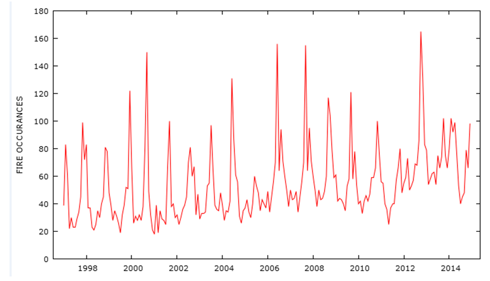 | Figure 1. Time series plot of Fire Outbreaks |
3.1. Sarima Model Estimation
The evidence of both seasonality and non-seasonality differenced to make the data stationary was based on logarithmical transformation of fire data. Also the seasonality and the non- seasonality of the series were affirmed from the oscillation of the ACF plot as depicted in Figure 2.The following spikes 12, 24, 36 and 48 were significant at the seasonal displayed in residual sample autocorrelation function and also a very dominant significant spike at lag 1 and 12 PACF plot in Figure 2. 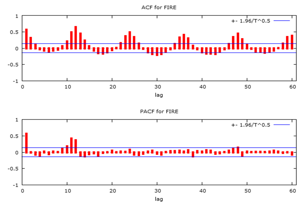 | Figure 2. Residual correlogram of the fire model |
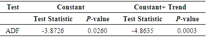
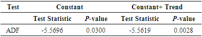
The ADF test shown in Table 2 revealed that the transformed seasonal differenced series was not stationary.Table 2. ADF test of seasonal differenced Fire Outbreaks
 |
| |
|
Therefore, due to the seasonality in the data, a logarithmic transformation was made to stabilize the data (stable variance). To check stationarity, the transformed fire series was seasonal differenced and tested at 5% level of significance. The transformed seasonal differenced fire outbreaks were again non-seasonal differenced. The ADF test in Table 3 affirms that the transformed seasonal and non-seasonal differenced fire outbreak is stationary.Table 3. ADF test of seasonal and non-seasonal differenced series
 |
| |
|
Furthermore, the stationarity of the series can also be confirmed from the time series plot of the transformed seasonal and non-seasonal differenced series. As shown in Figure 3, the series fluctuates about the zero-line confirming stationarity in mean and variance of the series.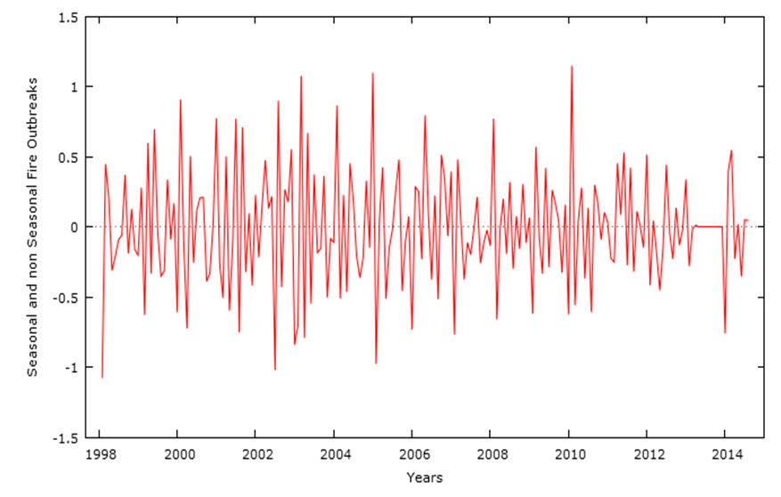 | Figure 3. Time series plot of first differenced series |
After the fire outbreaks order of integration has been obtained, the order of the Autoregressive and Moving Average for both non-seasonal seasonal components was determined. This was obtained from the ACF and PACF plots based on the Box and Jenkins (1976) approach.From Figure 4, the ACF plot have significant spike at the non-seasonal lag 1 and seasonal lag 12, with significant spikes at other non-seasonal lags. The PACF plot also has significant spikes at the non-seasonal lags 1, 2, 3 and 4 seasonal lags 12 and 36. The PACF plot also has significant spike at other non-seasonal lags. We identified candidate models for the fire outbreaks by using the lower significant lags of both the ACF and PACF and their respective seasonal lags.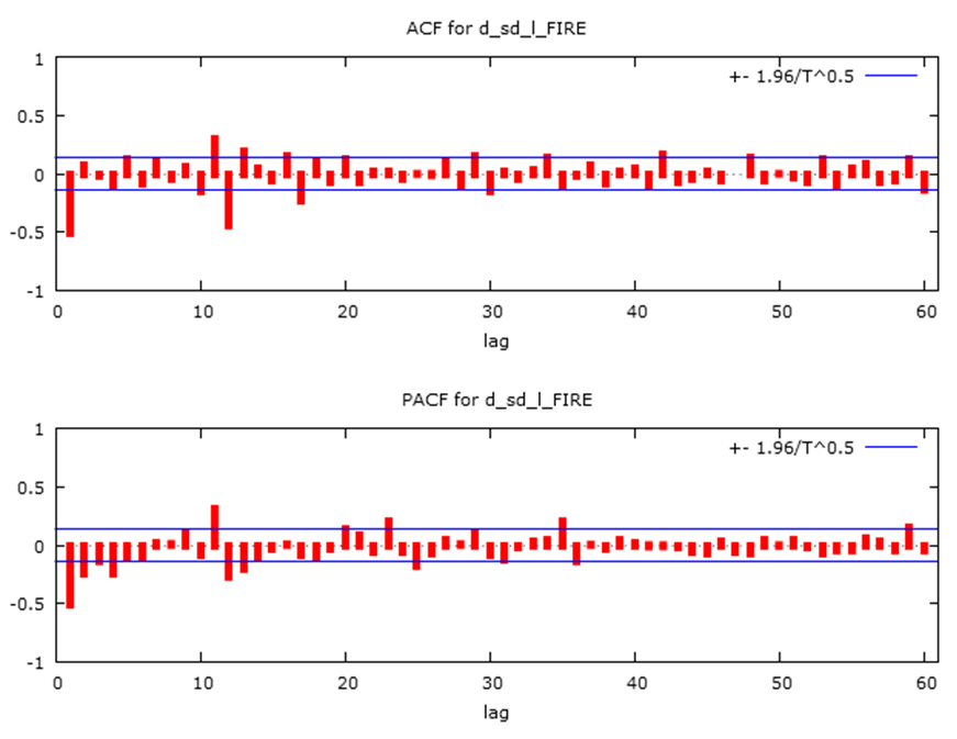 | Figure 4. ACF and PACF plot of differenced series |
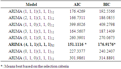
Table 4 below shows various candidate models identified and among these possible models presented in Table 4, ARIMA (4, 1, 1)(1, 1, 1)12 was chosen as the appropriate model that fit the data well because it has the minimum values of AIC and BIC compared to other models.Table 4. Candidate SARIMA Models
 |
| |
|
The estimation of parameters of our derived model is obtained by using the method of maximum likelihood shown in Table 5. The ARIMA (4, 1, 1)(1, 1, 1)12 model and can be expressed in terms of the lag operator as;  implies
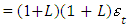
Table 5. Estimates of parameters for ARIMA (4, 1, 1)(1, 1, 1)12
 |
| |
|
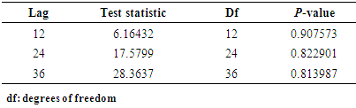
The observations of the p-values of the parameters of the model for both the non-seasonal and seasonal and Autoregressive and Moving Average components are highly significant at the 5% level. The model appears to be the best model among the proposed models.When fitting data in time series analysis, the best model selection is directly related to whether residual analysis is performed well. One important assumptions of good ARIMA model is that, the residual must follow a white noise process which implies zero mean, constant variance and uncorrelated residual. From the diagnostic plot in Figure 5, the standardized residuals revealed that the residuals of the model have zero mean and constant variance. Also, the ACF of the residuals shows that the autocorrelation of the residuals are all zero which implies that they are uncorrelated. Finally, in the third panel, the Ljung-Box statistic indicates that there is no significant departure from white noise for the residuals as the p-values of the test statistic clearly exceeds the 5% significance level for almost all lag orders.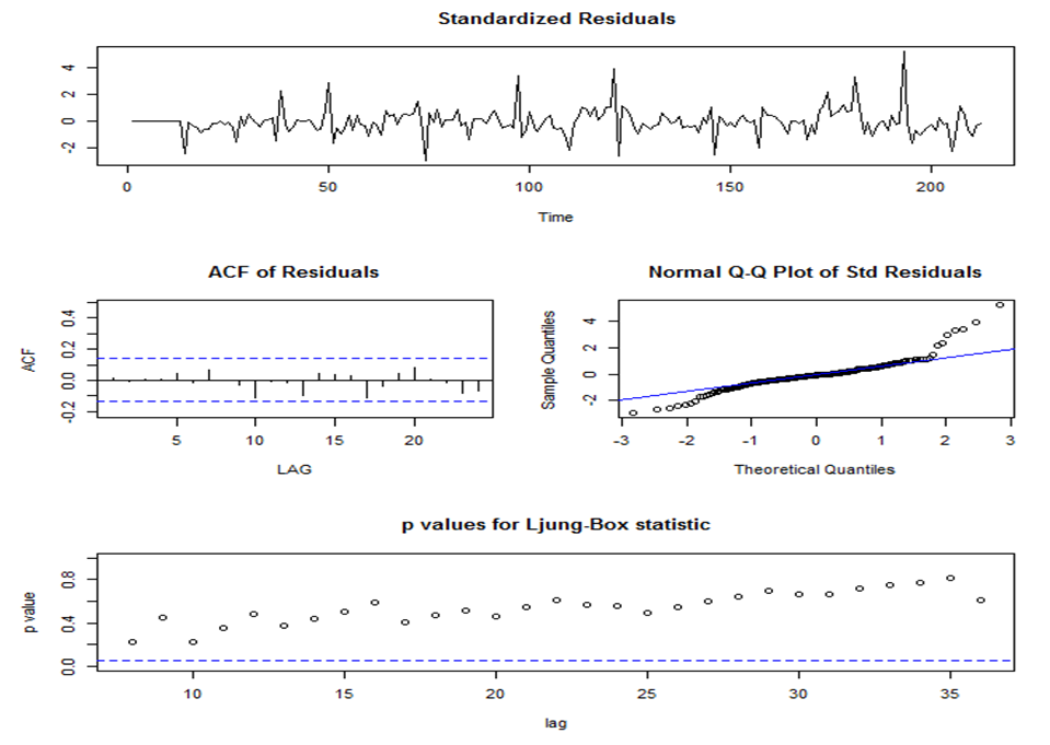 | Figure 5. Diagnostic plot of ARIMA (4, 1, 1)(1, 1, 1)12 |
To support the information depicted in Figure 6, the ARCH-LM test and t-test were employed to test for constant variance and zero mean assumption respectively. From the ARCH-LM test result shown in Table 6, we fail to reject the null hypothesis of no ARCH effect in the residuals of the selected model. Also, the t-test gave a test statistic of -1.3281 and a p-value of 0.1865 which is greater than the 5% significance level. Thus, we fail to reject the null hypothesis that the mean of the residuals is equal to zero. Hence, the selected model satisfies all the assumptions and it can be concluded that ARIMA (4, 1, 1)(1, 1, 1)12 model provides an adequate representation of the fire outbreaks.Table 6. ARCH-LM test of residuals of ARIMA (4, 1, 1)(1, 1, 1)12
 |
| |
|
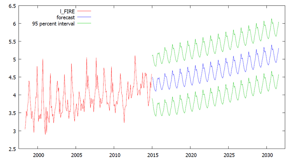 | Figure 6. Forecasting plot of ARIMA (4, 1, 1)(1, 1, 1)12 |
The graph below depicts the forecast of fire outbreaks from December, 2016. From the graph, there is an indication of an alternating increase pattern in fire outbreaks.
3.2. Conclusions
The forecasting of the number of fire outbreaks is important to fire stakeholders and management in Ghana. The forecasting model was developed to aid in the monthly prediction of the fire outbreaks.The model was the ARIMA (4, 1, 1)(1, 1, 1)12 model. The monthly forecasting model.ARIMA (4, 1, 1)(1, 1, 1)12 gives a non-seasonal autoregressive of order four (4), AR(4) which indicates that the future monthly fire outbreaks correlates with its fourth months. This as a result means that an increase or decrease in fire outbreaks in the fourth month will result in increase or decrease in fire outbreaks in the future and the differencing of order one, I(1) indicates the removal of linear tread in the data which makes it stationary. Also the non -moving average of order one, MA (1) indicates that the future monthly fire outbreaks errors depend on error term of its preview month.Furthermore, the seasonal autoregressive of order one, AR (1), indicates that the monthly future fire outbreaks correlates with its preview one-year monthly fire incidence and the seasonal moving average of order one MA (1) also indicates that the forecasting values of fire outbreaks depend on it past one year errors.The diagnostic checks on this model proved that the model was adequate for predicting the monthly number of fire outbreaks in Ashanti Region of Ghana. Hence, it was concluded that the model is good for forecasting fire outbreaks. The sixteen years forecast with this model revealed that the number of fire outbreaks will continue to increase with time. This continuous increase in the pattern of the number of fire outbreaks as evident from the forecast results could be a great danger to the economy of the country. The results achieved for fire forecasting will help to estimate, plan and manage fire related activities.
3.3. Recommendations
Following the outcome of this research work, the following recommendations were made;i. Stakeholders in fire management such as Ghana National Fire Service, Ghana police Service, insurance companies and other financial agencies should make use of this formulated SARIMA model for the purpose forecasting, mitigating and insuring against fire outbreaks in Ghana. ii. Stakeholders in fire management are concerned with developing effective means of managing fire. It is recommended that, they provide data on daily and weekly number of fire occurrences readily available to researchers. This would enable researchers to investigate within the month effects on the number of fire outbreaks.
References
| [1] | Aidoo, E., (2010). Modelling and Forecasting Inflation Rates in Ghana: An Application of SARIMA Models. Hogskolan Dalarna, School of Technology and Business Studies. Unpublished M. Sc. Thesis. |
| [2] | Asante, D., (2012). Regression Analysis on Fire Outbreaks. University for Development Studies, Department of Statistics, Navrongo. Unpublished BSc thesis. |
| [3] | Dickey, D. A., & Fuller, W. A., (1979). Distribution of the Estimators for Autoregressive Time Series with a Unit-root. Journal of the American Statistical Association, 74: 427-431. |
| [4] | Engle, R. F., (1982). Autoregressive Conditional Heteroscedasticity with estimates of the variance of United Kingdom Inflation. Econometrical, 50: 987-1007. |
| [5] | Ghana News Agency (Accessed: December 2011). Cost of Damage by fire outbreak. www.ghananewsagency.org. |
| [6] | Halim, S., & Bisono, I.N., (2008). Automatic Seasonal Autoregressive Moving Average Model and Unit Root Test Detection. International Journal of Management Science and Engineering Management, 3(4): 266-274. |
| [7] | Lang, M., Kunovac, D., Basac, S., & Staudinger, Z., (2008). Modelling of Currency outside Banks in Croatia. Croatian National Bank Working Papers W-17. |
| [8] | Keane, Robert E.; Morgan, Penny M.; Dillon, Gregory K.; Sikkink, Pamela G.; Karau, Eva C.; Holden, Zack A.; & Drury, Stacy A., (2013). A Fire Severity Mapping System forReal-Time Fire Management Applications and Long-Term Planning: The FIRESEV project JFSP Research Project Reports. Paper 18. |
| [9] | Ljung, G. M., & Box, G. E. P., (1978). On A Measure of Lack of Fit in Time Series Models. Biometrika, Journal of Econometrics, 65:297-303. |

 Abstract
 Reference
 Full-Text PDF
 Full-text HTML