Md. Shahajada Mia1, Md. Siddikur Rahman2
1Department of Statistics, Pabna University of Science and Technology, Pabna, Bangladesh
2Department of Statistics, Begum Rokeya University, Rangpur, Bangladesh
Correspondence to: Md. Shahajada Mia, Department of Statistics, Pabna University of Science and Technology, Pabna, Bangladesh.
| Email: |  |
Copyright © 2019 The Author(s). Published by Scientific & Academic Publishing.
This work is licensed under the Creative Commons Attribution International License (CC BY).
http://creativecommons.org/licenses/by/4.0/

Abstract
Exchange rate is the price of one currency in terms of another currency. Modelling exchange rate volatility can play an important role in macroeconomic management for stability and growth. This paper examine the forecasting accuracy of ARCH family models for the monthly BDT/ USD exchange rate data from Bangladesh Bank over the period from August, 2004 to April, 2019. To find an appropriate model, several model selection criterion: Akaike information criteria (AIC) and Schwarz information criteria (SIC) and for measuring accuracy Root mean squared error (RMSE), Mean absolute error (MAE), Mean absolute percentage error (MAPE) and Theil inequality (TI) are used. Evaluation of models through these criteria suggest that GARCH (1,1) model is the best model for forecasting the monthly exchange rate volatility of Bangladesh and successfully overcome the leverage effect in the exchange rate.
Keywords:
Exchange rate, ARIMA, Volatility, ARCH family models
Cite this paper: Md. Shahajada Mia, Md. Siddikur Rahman, Evaluating the Forecast Accuracy of Exchange Rate Volatility in Bangladesh Using ARCH Family of Models, American Journal of Mathematics and Statistics, Vol. 9 No. 5, 2019, pp. 183-190. doi: 10.5923/j.ajms.20190905.01.
1. Introduction
Exchange rate is the price of one currency in terms of another currency. Over the last few decades, exchange rate movement and fluctuations has become an important subject of macroeconomic analysis and have received a great deal of interest from academics, financial economists and policy market. In an open and deregulated economic environment, exchange rates can play an important role in macroeconomic management for stability and growth. Depreciated exchange rate would reduce imports and increase exports and thereby contracting a country’s trade deficit. The rates are inherently noisy, non-stationary and deterministically chaotic. These characteristics suggest that there is no complete information that could be obtained from the past behavior of such markets to fully capture the dependency between the future rates and that of the past. As a result, the appropriate prediction of exchange rate is a crucial factor for the success of many businesses and fund managers. This research aims to analyze and compare the capacity of different mathematical models such as ARCH, GARCH, EGARCH, IGARCH and TARCH models.
2. Literature Review
Quite a few studies have forecast the exchange rates (BDT vs. USD) of Bangladesh by econometric models. Different methods are used to predict exchange rates. These methods are distinguishable from each other by what they hold to be constant into the future. These methods includes moving average (MA), autoregressive (AR), Exponential smoothing, autoregressive integrated moving average (ARIMA), vector autoregressive (VAR). Well known and frequently applied models to estimate exchange rate volatility are the autoregressive conditional heteroscedasticity (ARCH) model advanced by Engle (1982) and generalized autoregressive conditional heteroscedasticity (GARCH) model developed independently by Bollerselv (1986) and Taylor (1986). Other models are: EGARCH model was proposed by Nelson (1991) and TARCH model introduced by Glosten, Jaganathan, and Runkle (1993) and Zakoïan (1994).Mandelbrot (1963) and Fama (1965) have shown that the time series of exchange rates are generally characterized by conditional heteroscedasticity, leptokurtic and volatility clustering. Various ARCH models have been applied by researchers to analysis the volatility of exchange rates in different countries. Such studies are: (Benavides, 2006) analyses the volatility forecast for the Mexican Peso- U.S. Dollar exchange rate, (Alam et. Al., 2012) analyses the exchange rates of Bangladeshi Taka (BDT) against the U.S. Dollar for the period of July 03,2006 to April 30,2012, (Musa et.al, 2014) forecast the exchange rate volatility between Naira and US Dollar using GARCH models. Ng and McAleer (2004) used simple GARCH (1,1) and TARCH(1,1) models for testing, estimation and forecasting the volatility of daily returns in S&P 500 Composite Index and the Nikkei 225 Index. Their empirical results indicate that TARCH (1,1) model seems to perform better with S&P 500 data, whereas the GARCH(1,1) model is better in some cases with Nikkei 225.
3. Material and Methods
3.1. Data Source
For this article, the data of monthly exchange rates of Bangladesh (BDT vs. USD) has been collected from Bangladesh Bank over the period from August, 2004 to April, 2019. So there are total of 176 monthly observations.
3.2. Methodology
To determine the appropriate model for predicting the exchange rates of Bangladesh at first the stationary of the data will be checked using graphically, and unit root test i.e. ADF (Augmented Dickey-Fuller) test and Philips Perrons (PP) test are used here. If the series is stationary then using the ordinary least square (OLS) method foreign exchange rate moving pattern of Bangladesh is estimated. The foreign exchange rate moving pattern may autoregressive (AR) or moving average (MA) or combination of AR and MA (ARMA) or autoregressive integrated moving average (ARIMA).The AR (p) model can written as  | (1) |
The MA (q) model can be written as  | (2) |
The combination of AR (p) and MA (q) model i.e. ARMA (p, q) model is expressed in the following form: | (3) |
Where,  and
and  are the actual value and random error at time period t respectively;
  (i=1,2,3,…….,p) and
  (j=1,2,3,……..,q) are model parameters. The integer’s p and q are referred to as order of autoregressive and moving average respectively. Random error term
  are assumed to be independently and identically distributed (i.i.d) with mean zero and constant variance
  . Using backward shift operator the ARMA (p, q) model can be written in the following form
 | (4) |
Where  and
and  .If the time series is not stationary, then we convert it to stationary by taking it differencing. If d is the order of difference series then the ARIMA (p, d, q) model can be written as
 | (5) |
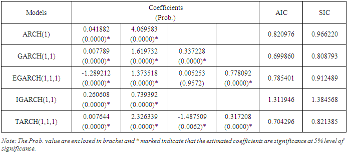
Afterwards heteroscedasticity test (ARCH LM test) on residuals of exchange rates are used to find the significance of the ARCH effect. If the ARCH effect is significant, several ARCH models like as Autoregressive conditional heteroscedasticity (ARCH), Generalized Autoregressive conditional heteroscedasticity (GARCH), Exponential generalized autoregressive conditional heteroscedasticity (EGARCH), Integrated generalized autoregressive conditional heteroscedasticity (IGARCH) and Threshold autoregressive conditional heteroscedasticity (TARCH) models are tested and compared based on the lowest values of Akaike information criteria (AIC) and Schwarz information criteria (SIC). Among them ARIMA are used as a mean model and the remaining model like as ARCH, GARCH, EGARCH, IGARCH and TARCH are used a variance model to forecast the volatility of exchange rate.
3.3. Forecasting Performance
In this article, to identify the best model for forecasting the exchange rate of Bangladesh we have used several measured such as Root Mean Square Error (RMSE), Mean Absolute Error (MAE), Mean Absolute Percentage Error (MAPE) and Theil Inequality (TI).• The Root Mean Square Error:  • The Mean Absolute Error:
 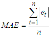 • The Mean of the Absolute Percentage Error:
 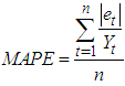 • Theil’s inequality coefficient: TI = (RMSE of the forecasting model) / (RMSE of the actual model)Where,
  is the forecast error in time period t.
 is the actual value in time period t.n is the number of forecast observations in the estimation period.The smaller values of MAE, RMSE and MAPE, the better the model is considered to be. A theil’s inequality is closer to 0 indicates that better fit the model.
4. Results and Discussion
4.1. Stationary Test and ARIMA Model Selection
Before modelling the exchange rate first we confirmed the series is stationary. Time series plot and unit root test (such as ADF and PP test) are used to check the series stationary or not. The time series plot of exchange rate series shown in Figure 1(a) which shows an upward trend suggesting that the exchange rate series is non stationary since the mean of exchange rate has been changing over the periods but the 1st differencing series of exchange rate shown in Figure 1(b) suggest the series stationary since its mean and variance are constant over time.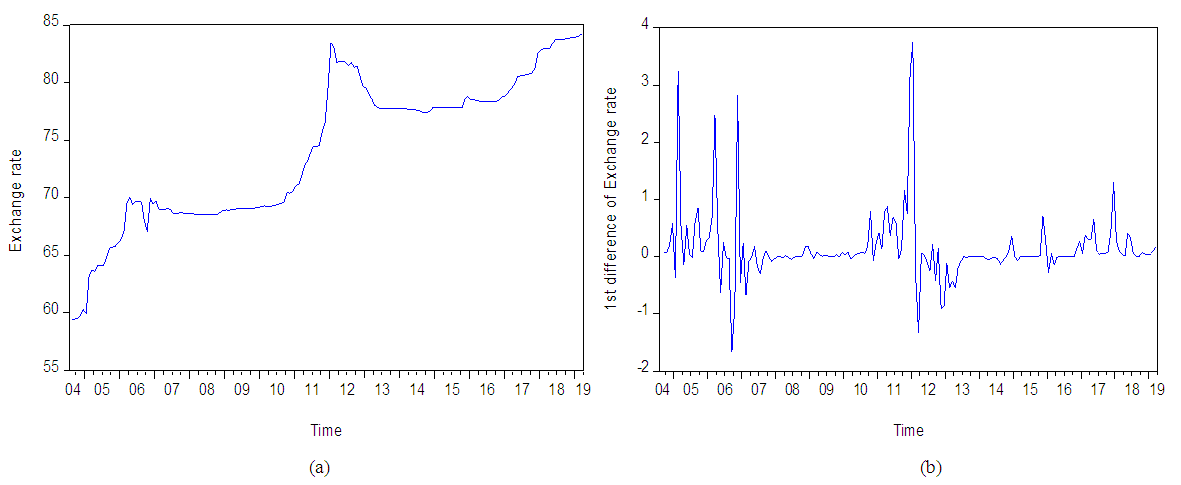 | Figure 1. Time series plot of monthly exchange rate (a) and First difference of exchange rate series (b) |
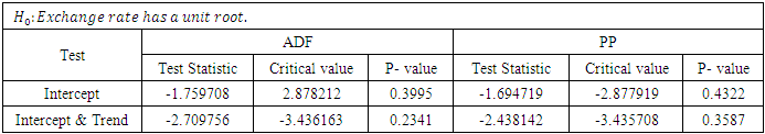
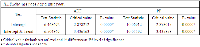
To confirm this we have used here Augmented Dickey Fuller (ADF) and Philips-Perron (PP) test. ADF and PP test suggest that the original series is insignificant (Table-1) but 1st difference series is highly significant (Table-2) at 5% level of significance. Therefore the exchange rate series is non-stationary but after the non-seasonal 1st differencing, both test suggest that the series is stationary. Therefore for further analysis, we used the data in first difference.Table 1. Unit root test of exchange rate series
 |
| |
|
Table 2. Unit root test of exchange rate series
 |
| |
|
After the series has been stationarized by 1st differencing, the next step in fitting an ARIMA model is to determine how many AR or MA terms are needed to correct any autocorrelation that remains in the second differenced series. Therefore, the order of AR and/or MA terms that are needed to fit a model are tentatively identified by looking the ACF and PACF plots of the 1st differenced series. Since after 1st difference we get a stationary series so the order of d will be 1. It is obvious from the sample ACF of the 2nd difference series (shown in figure 2) the most dominating spike at lag 1 are statistically significant for ACF and PACF. Therefore based on the ACF and PACF plot we have selected ARIMA (1,1,1) as the best model among other ARIMA models as a mean model to forecast the exchange rate and this model are selected also based on the automatic ARIMA model on the basis of lowest values of AIC and SIC.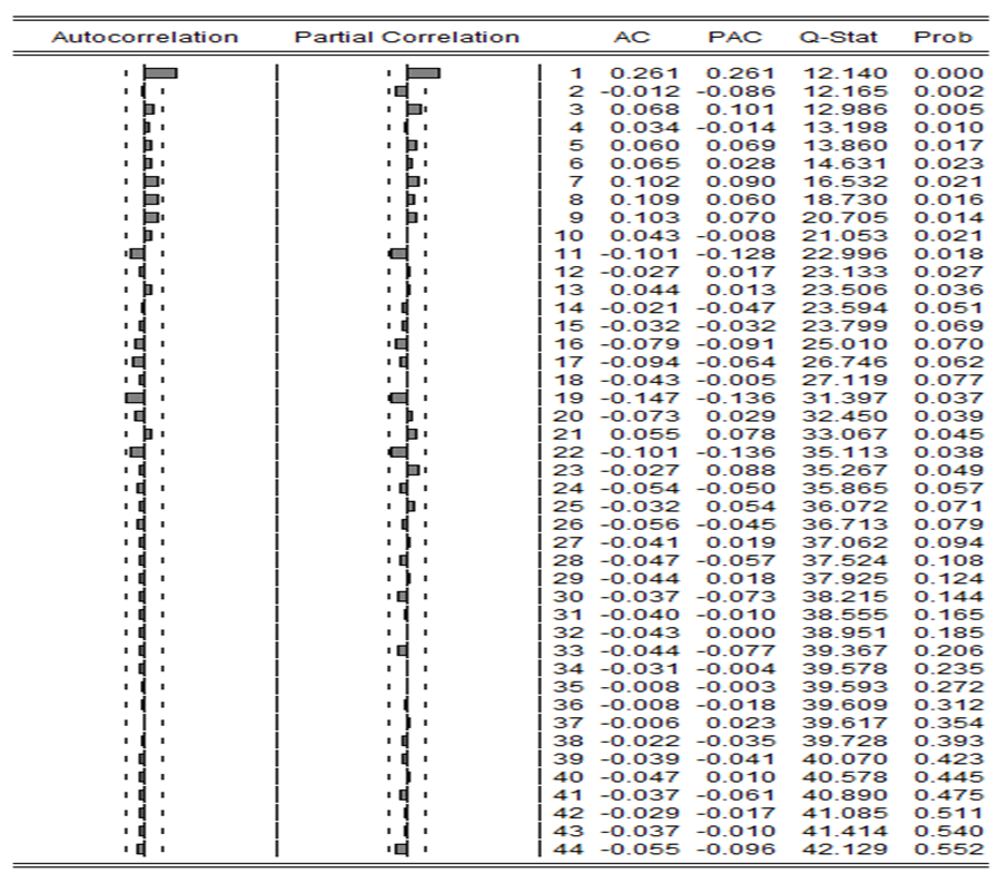 | Figure 2. Correlogram of 1st difference of exchange rate series |
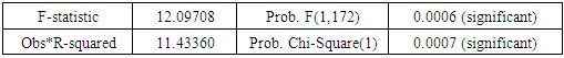
After fit the model we have check that if there is an ARCH effect in this model by using residual plot and ARCH LM test.Figure-3 shows that the volatility has changed after some periods i.e there may be an ARCH effect of the series. To make sure, we will run heteroscedasticity test. Table-3 suggest that there is an ARCH effect since its p-value is less than 5% level of significance. Since ARCH effect is significant therefore ARCH family of models can be estimated.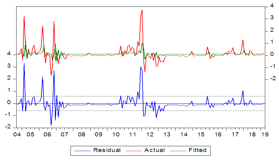 | Figure 3. Residual plot of ARIMA (1,1,1) model |
Table 3. ARCH LM test
 |
| |
|
4.2. ARCH Family Models Analysis and Comparisons
In our study we have developed different ARICH family models i.e.ARCH, GARCH, EGARCH, IGARCH and TARCH and one of among them select to better forecast the exchange rate volatility based on the Akaike information criteria (AIC) and Schwarz information criteria (SIC) values. Table-4 suggest that among all models GARCH (1,1) is the best model since it has lowest value of AIC and SIC.Table 4. Comparisons of different ARCH family of models
 |
| |
|
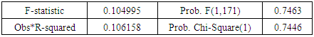
The plot of ACF of residual and ARCH LM test of residual of the selected GARCH (1,1) model shown in figure-4 and table-6 respectively (see appendix). They suggest that there is no serial correlation in the residuals since all the p values are less than 5% and there is no ARCH effect in the model respectively. Therefore we have a good model GARCH (1,1) for forecasting the volatility of exchange rate.
4.3. Forecasting Accuracy Comparisons
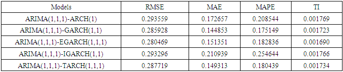
To check the forecasting accuracy of different models, we have used 21 observations of exchange rate series from the period August, 2017 to April, 2019. The forecasting performance of different models are compared on the basis of root mean square error(RMSE), mean absolute error(MAE), mean absolute percentage error(MAPE) and Theil inequality (TI). Table-5 shows the forecasting comparisons of different model based on RMSE, MAE, MAPE and TI and suggest that ARIMA(1,1,1)-GARCH(1,1) is the best model since it has lowest values of RMSE, MAE, MAPE and TI are close to 0. Figure-5 (shown in appendix) shows the forecasted values and confidence intervals for different models. Therefore this paper suggest that ARIMA (1,1,1)-GARCH (1,1) is better model to forecast the exchange rate of Bangladesh.Table 5. Comparisons of different models in out of sample forecasting accuracy
 |
| |
|
5. Conclusions
In this paper we have built a model to forecast the exchange rate of Bangladesh. Since volatility of exchange rate has a significant impact on trade and remittance and consequently on the whole of economy. So it is important to select an appropriate model to forecast the volatility of the exchange rate. Monthly average exchange rates of Bangladesh for the period from August, 2004 to April, 2019 are used for this study. After checking the stationary of the series by graphical method and unit root test we have select ARIMA (1,1,1) as a mean model for this study. Then this study tried to model the volatility of exchange rate using ARCH, GARCH, EGARCH, IGARCH and TARCH models. Among ARCH family models, GARCH (1,1) is found to be the best model since it has the lowest values of AIC and SIC compared to other models. In out of sample forecasting accuracy, ARIMA (1,1,1)-GARCH (1,1) is selected as a best model compared to others since it has the lower values of RMSE, MAE, MAPE and TI than others model. Finally the papers conclude that exchange rate volatility and forecasting can be adequately modeled by the ARIMA (1,1,1)-GARCH (1,1) model.
Appendix
Table 6. ARCH LM test of ARIMA (1,1,1)-GARCH (1,1) model
 |
| |
|
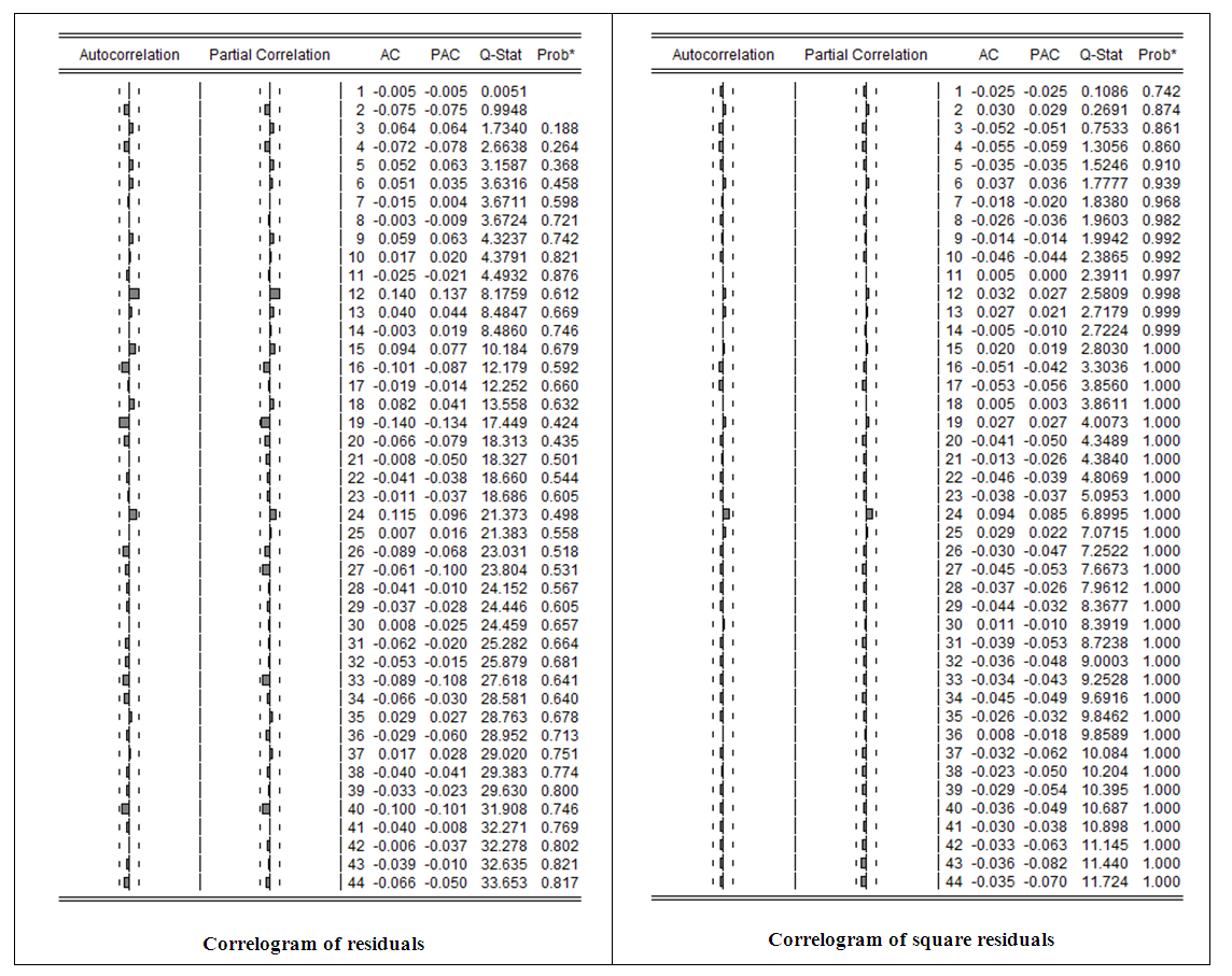 | Figure 4. Serial correlation of ARIMA (1,1,1)-GARCH(1,1) model |
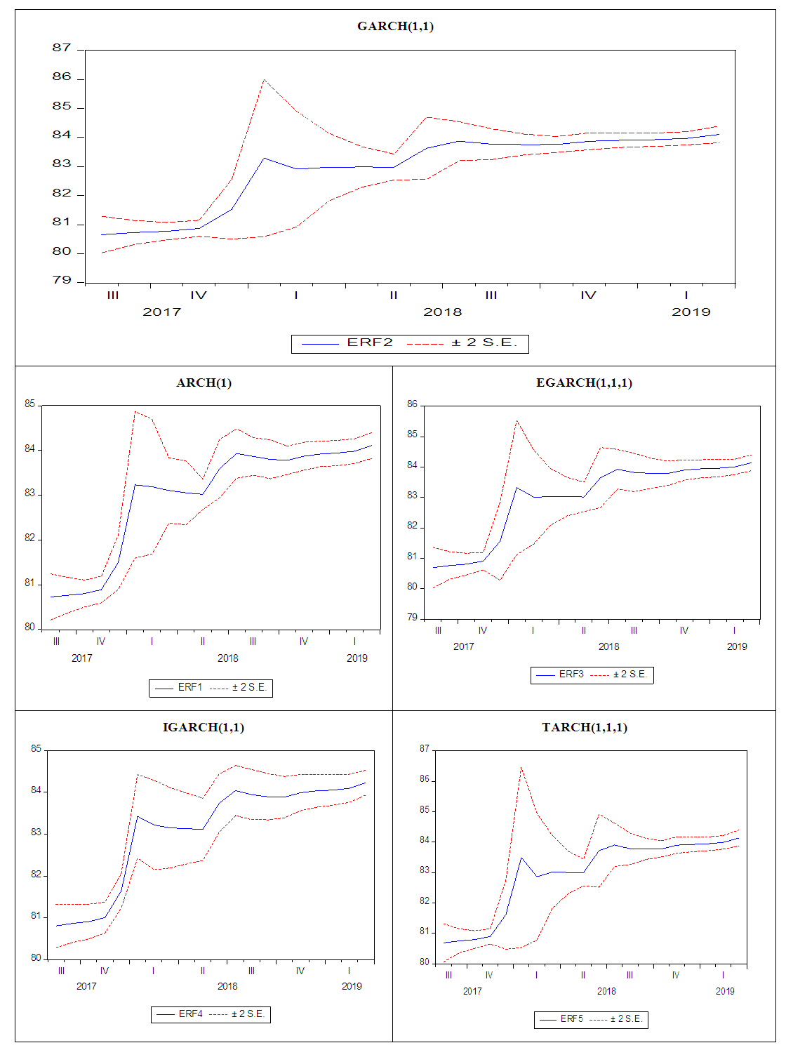 | Figure 5. Forecasting exchange rate volatility using different models |
References
| [1] | Alam, Z., Rahman, A. (2012) “Modelling Volatility of the BDT / USD Exchange Rate with GARCH Model“, International Journal of Economics and Finance 4, pp. 193 – 204. |
| [2] | Baillie, R.T., Bollerslev, T. (2002). The massage in daily exchange rates: A conditional variance tale. Journal of Business and Economic Statistics, 20(1), pp. 60-68. |
| [3] | Benavides, Guillermo. (2006) “Volatility Forecasts for the Mexican Peso - U.S. Dollar Exchange Rate: An Empirical Analysis of GARCH“, Option Implied and Composite Forecast Models, Banco de Mexico, Research Document , pp. 1 – 39. |
| [4] | Bollerslev, T. (1986) “Generalized Autoregressive Conditional Hetroscedasticity”, Journal of Econometrics 31, pp. 307 – 327. |
| [5] | Dickey, D., Fuller, W. (1981) “Distribution of the estimators for autoregressive time series with a unit root”, Econometrica Journal 49, pp. 1057 – 72. |
| [6] | Engle, R. F. (1982) “Autoregressive Conditional Heteroscedasticity with Estimates of the Variance of United Kingdom Inflation”, Econometrica 50, pp. 987 – 1008. |
| [7] | Fama E. F. (1965), “The behavior of stock market prices”, in Journal of Business, n. 38, pp. 34–105. |
| [8] | Glosten, L, Jagannathan, R., Runkle, D. (1993) “On the relationship between the Expected Value and the Volatility of the Nominal Excess Return on Stocks”, Journal of Finance 48, pp. 1779 – 1802. |
| [9] | Mandelbrot B. B. (1963), “The variation of certain speculative prices”, in Journal of Business, n.36, pp.394–419. |
| [10] | Musa, Y., Tasi’u, M., Abubakar, B. (2014) “Forecasting of Exchange Rate Volatility between Naira and US Dollar Using GARCH Models“, International Journal of Academic Research in Business and Social Sciences, ISSN: 2222 - 6990, 4, 7, pp. 369 – 381. |
| [11] | Nelson, Daniel B. (1991) “Conditional Heteroskedasticity in Asset Returns: A New Approach”, Econometrica 59, 2, pp. 347 – 370. |
| [12] | Ng, H. G. and McAleer, M. (2004), “Recursive Modelling of Symmetric and Asymmetric Volatility in the Presence of Extreme Observations”, International Journal of Forecasting, 20:115-129. |
| [13] | Sayed Hossain, Hossain Academy, accesed 11 January, 2016, http://www.sayedhossain.com. |
| [14] | Taylor M. (2009), Purchaising Power Parity and Real Exchange Rates, Routledge. |
| [15] | Zakoïan, J. M., “Threshold Heteroskedastic Models”, Journal of Economic Dynamics andcontrol18, pp. 931-944. |

 Abstract
 Reference
 Full-Text PDF
 Full-text HTML