Nwakuya M. T., Biu E. O.
University of Port Harcourt, Rivers State, Nigeria
Correspondence to: Nwakuya M. T., University of Port Harcourt, Rivers State, Nigeria.
| Email: |  |
Copyright © 2019 The Author(s). Published by Scientific & Academic Publishing.
This work is licensed under the Creative Commons Attribution International License (CC BY).
http://creativecommons.org/licenses/by/4.0/

Abstract
This study examines the within-group and first difference fixed effect models using panel data set. Panel data on GDP, inflation, trade, civil-liability and population were collected across six African countries between 1972 and 1991, the data is an inbuilt R data found in amelia package. Performance of these fixed effect models were compared in terms of fitness using R- squared and relative efficiency. Results were generated using R software. Finding shows that in the within-group model, trade was the only independent variable that contributes significantly to GDP but in the first difference model both trade and population contributed significantly to GDP. The finding also reveals that within group model had a better fit with an R2 of 0.77317 as compared to first difference model which reported R2 of 0.75472. The relative efficiency was determined to be 1.3 showing that relative to within-group model the first difference model is preferred.
Keywords:
Within-Group Model, First Difference Model, Panel Data, Relative efficiency and Fixed Effect
Cite this paper: Nwakuya M. T., Biu E. O., Comparative Study of Within-Group and First Difference Fixed Effects Models, American Journal of Mathematics and Statistics, Vol. 9 No. 4, 2019, pp. 177-181. doi: 10.5923/j.ajms.20190904.04.
1. Introduction
1.1. Panel Data
In statistics and econometrics, Panel Data or longitudinal data are multi-dimensional data involving measurements over time. Panel Data refers to a data set containing observations on multiple phenomena over multiple time periods. Thus it has two dimensions: spatial (cross sectional) and temporal (time series). In general, we have two panels; micro and macro panels. Surveying (usually a large) sample of individuals or household or firms or industries over (usually a short) period of time yields micro panel whereas macro panel consist of survey over (usually a large) number of years.Panel data are more informative (more variability, less co-linearity, more degrees of freedom) estimates are more efficient. It minimizes bias due to aggregation. It allows the study of individual’s dynamics (e.g separating age and cohort effect). It also allows for the control for individual’s unobserved heterogeneity, though it increases the complexity of the analysis.The general panel data regression model is given as  | (1) |
Where i=1, 2... N stands for ith cross-sectional units (continues, family, friends)t = 1, 2,... T stands for tth period Yit = The dependent or response variableXit = Independent variables β0 = regression constantβi = regression coefficient eit = the error term and, 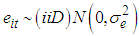 The panel data set structure can be in long format or wide format. Representing panel data in long format is much more common than using the wide format because it serves storage space. This is due to the fact that wide format will have lots of sparse cells wasting storage space depending upon the relative size of space and time ie short or long panels. In a short panel, the number of time periods (T) is less than the number of cross-section (T<N) and in a long panel T>N.Panel data has two important models; fixed effects and random effect model. In this work we focused on fixed effect model.
1.2. Fixed Effect Model
In fixed effects model all the factors are being considered fixed. The “effect” referred to in such a model represent measures of the influence that different levels of the factor have on the dependent variable and our conclusion cannot be extended to similar factors that were not explicitly considered. Fixed effects model in panel data assumes differences in constant across groups or time periods.The fixed effect model specifies: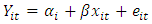 | (2) |
For i=1… N, t=1…TWhere the individual l- specific effect  measures unobserved heterogeneity that is possibly correlated with the regressorsXit = one independent variableΣit = errors term nd (0, δ2)β1 = coefficient of that one independent variable Fixed effect controls for all-time-invariant differences between the individuals, so the co-efficient of the estimated coefficient of the fixed effects model cannot be biased because of omitted time-invariant characteristics (culture, religion, gender, race etc).Panel data is said to be very informative and it estimates are efficient in, that it helps to reduce bias. However, considering of balanced and unbalanced data over the years scholars and researches have continued to argue as to which fixed effect model is the best. It is in the light of these that this study seeks to apply two different fixed effects models in a balanced data to ascertain the model efficiency and appropriateness. This research work aims at investigating the within group and first difference fixed effect models. The objectives include to determine the relative efficiency of the two methods and comparison of the two methods.
2. Literature Review
Cheng Hsiao has made significant and important contributions to panel econometrics, both methodologically and applied. His magisterial 1986 monograph is a long standard reference and popular graduate text. Hsiao provides applied examples which greatly enhance the reader’s understanding and intuition. He has added new chapters on nonlinear panel models of discrete choice and sample selection and included new material on the Bayesian treatment of estimation and more dynamic models.When Cheng Hsiao’s first edition of panel data was published, there were 29 studies listing the words “panel data or longitudinal data” according to social science citation index. By 2003, there were 580 and in 2004 there were 687 and by 2005, there were 773 studies.Clark (2003) through psychological evidence from panel data, investigated unemployment as a social norm in the labour market status. He used panel data to test for social norms in labour market status. The unemployed well-being was shown to be strongly positively correlated with reference group unemployment.Panel date showed that those whose well-being fell the most on entering unemployment are less likely to remain unemployed. These findings suggest a psychological explanation of both unemployment polarization and hysteresis based on the utility effect of a changing employment norm in the reference group.Mehdi and Fillipini (2003) examined the regulation and measurement of cost efficiency using panel data models. They examined the application of different parameter methods to measure cost efficiency of electricity distributes utilities. The cost frontier model was estimated using four methods; Ordinary least square, Fixed effects, Random effects and Maximum likelihood Estimation. These methods were applied to a sample of 59 distribution utilities in Switzerland. Results point to some advantages of fixed effects model in the estimation of cost function characteristics. The results also suggested that bench making methods can be used as a control instrument in order to narrow the information gap between the regulator and regulated companies. Bench making methods are methods hereby all comparisons are made in relation to a particular category.Hsiao et al (2007) propose limited information test to check for selection issues in addition to testing for sample selection, a number of studies have addressed the issue of treatment of unbalanced panels in the presence of selection bias.Nwakuya and Ijomah (2017) in their study investigated the fixed effect model versus the random effect model, using an economic panel data set in the analysis the fixed effect model was found to be most appropriate.
3. Method of Data Analysis
3.1. Fixed Effects Model Approach
The fixed effects model approach depends on the different parameter assumptions we make about the constant and regression co-efficient of the models. The fixed effect model has many models, but for this work we focused on two of the models namely within group and first difference models. The data for this work is a secondary data gotten from R inbuilt data set, it is called Africa. The fixed effect models are designed to study the causes of changes within an entity. A time-invariant characteristics cannot cause such a change because it is a constant for each individual. An assumption of fixed effect model is that those time invariant characteristics should not be correlated with other individual characteristics.
3.2. Within Group Fixed Effect Model
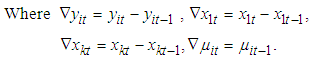
One of the models of fixed effect is the least square dummy variable model, it’s the simplest method of isolating individual or time specific effect in a regression model, Nwakuya & Ijomah (2017), but its drawback is that, it is not feasible when the number of explanatory variable is large. To estimate fixed effect model with large number of individuals the within group fixed effect model is adopted. The within group fixed effect model eliminates the fixed effect, by expressing the values of the dependent and explanatory variables for each observation as deviations from their respective mean values, Gujarati and Porter (2009).Given equation (1), averaging the observation across time using the assumption on time-invariant parameter.
 | (3) |
Where 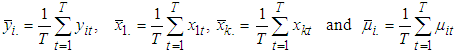 Now subtract equation (5) from (4).
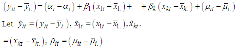 Hence, the equation becomes
 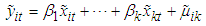 | (4) |
In matrix form | (5) |
Equation 5 above is known as the within transformed model, it has eliminated the unobservable across-group differences. The within-group fixed effect model estimate of β is known as the within estimator, and is given as: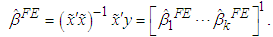 | (6) |
The within estimator’s explanatory value is derived from the co-movements of y around its individual-specific mean with x around its individual-specific mean. The estimator basically borders about how the variations around those mean values are correlated, Wooldridge (2006).
3.3. First Difference Fixed Effect Model
The first difference estimator wipes our time invariant variables using the repeated observations over time, Bruce E. H. (2016). First difference estimator is also an approach for addressing the problem of omitted variables in a panel data analysis.From equation (1), we have: Lagging equation (1) one period, we have;
 | (7) |
Subtraction equation (7) from equation (1), we have;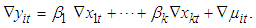 | (8) |
 The first difference transformation eliminates the unobserved effect of the parameters and also causes the loose of the first time period for each cross section and we have T-1 time periods for each cross section, rather than T, Wooldridge (2001).The β estimate for the first difference model in matrix form is given by:
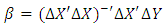 | (9) |
3.4. Relative Efficiency
The relative efficiency of two procedures is the ration of their efficiencies. It is usually a comparison made between a procedure and a notional procedure (say one with less variance).Given two unbiased estimators  the efficiency of
  relative to
  is given by;
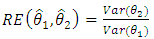 | (10) |
This can be used to decide which of the two models will be preferred relative to the other. Given equation (10), Lebanon (2006), stated that if relative efficiency is greater than one i.e  , then
  is preferred but if
  then
then  is preferred.
4. Results and Discussions
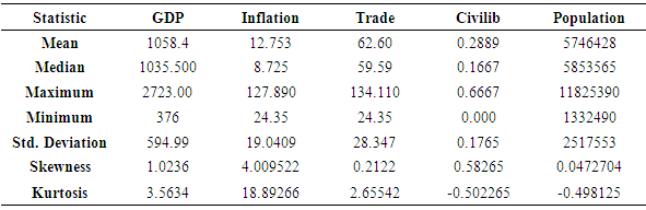
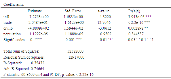
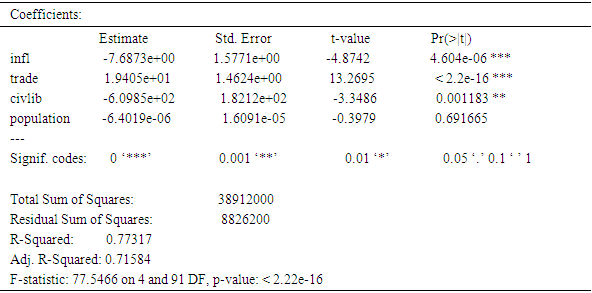
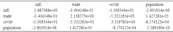
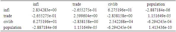
The result of the fixed effects based on first difference and within- group models are presented here. The results includes; descriptive statistics, parameter estimates for both models and results of the comparison based on their relative efficiency. Table 4.1 presents summary of the descriptive statistics for the research variables (GDP, inflation, trade, civlib and population). Result reveals that among the variables, Inflation reveals highest kurtosis as compared to the other variables.Table 4.3 shows results from within- group model, with R-squared of 0.77317 which implies that 77.317% of the variation in GDP across the selected countries was explained by Inflation, trade, Civil-liability. The parameter estimated in table 4.5 indicates, while table (4.2) shows results from first difference model with R-squared of 0.75472 meaning that the model accounted for 75.472% of the variation in GDP, its parameter estimates indicates that as inflation and civiliability increases, GDP decreases while as trade and population increases, there is an improvement in GDP. Test for autocorrelation using Watson test showed no evidence of autocorrelation. Table 4.4 and 4.5 shows the variance covariance matrix for within-group and first difference models respectively. The comparison was done in terms of fitness and relative efficiency.Table 4.1. Summary of the Descriptive Statistics for the Variables
 |
| |
|
Table 4.2. Results from first difference fixed effect Model
 |
| |
|
Table 4.3. Results from within group
 |
| |
|
Table 4.4. Variance covariance matrix of within group
 |
| |
|
Table 4.5. Variance covariance matrix of first difference
 |
| |
|
The total variance is the sum of the diagonal matrix, and we have that for within group the total variance ie  = 33172.46 and total variance for first difference ie
  =25428.114.Therefore;Relative Efficiency = 1.3 in terms of relative efficiency the first difference is preferred.
5. Conclusions
This research work has compared the performance of first difference model and within group model in a panel data based on relative efficiency. The result has shown that the within-group model had a better fit, in terms of the explained percentage of variation of the GDP by the predictor variables considered in this work, but we went further to compare the models based on the quality of their estimators. The comparison indicated that even though the within-group had a better model fit the first difference model is a more preferred model in terms of the quality of their estimators. This research work has been able to show that a model with a better model fit does not necessarily give better estimators. All analysis were done in R.R codes:#calculating kurtosis, standard deviation and skewness>skewness(africa$population)>kurtosis(africa$population)>sd(africa$population)#above is repeated for every predictor# first difference model>fd3<- plm (gdp_pc ~ infl + trade + civlib + population – 1,data=Africa,model=’fd’)# within-group model>fd2<-plm(gdp_pc~infl+trade+civlib+population-1,data=africa,model="within")#variance covariance for within-group Vcov(fd3)#trace of variance covariance matrix = total variance for within-grouptrm2<-sum(diag(vcov(fd3)))#variance covariance for first difference Vcov(fd2)#trace of variance covariance matrix = total variance for first differencetrm1<-sum(diag(vcov(fd2)))#Relative efficiencytrm2/trm1
References
| [1] | Anderson T.W. and Hsiao C. (1981), Estimation of Dynamic Models Error Components. Journal of the American Statistical Association, 76, 598(606). |
| [2] | Bruce E. H. (2016), Econometrics, University of Wisconsin press. |
| [3] | Clark A. E. and Etile F. (2003), Heterogeneity in Reporting well-being. Evidence and inferences in Econometrics. New York Oxford University Press. |
| [4] | Gujarati D. N. and Porter D. C. (2009), Basic Econometrics, McGraw-Hill Companies Inc., pp 599-601. |
| [5] | Lebanon G. (2006), Relative Efficiency, Efficiency and the Fisher Information, www.cc.gatech.edu/~lebanon/notes/efficiency.pdf. |
| [6] | Mehdi, F. and Fillipine, M. (2003), Journal on “Regulation and Measuring cost Efficiency with Panel data models”. |
| [7] | Hsiao C. (2007), Panel Data Analysis-Advantages and Challenges. Econometrics society Monographs 16(1) pp1-22. |
| [8] | Hsiao C. (2003), Analysis of Panel Data 2nd edition, Econometrics society Monographs 36, New York Cambridge University Press. |
| [9] | Nwakuya M. T. and Ijomah M. A. (2017), Fixed Effects Versus Random Effects Modeling in a Panel Data Analysis: A Consideration of Economic and Political Indicators in Six African Countries, International Journal of Statistics and Applications, Vol7 (6), pp 275-279. |
| [10] | Woooldridge J. M. (2001), Econometrics Analysis of Cross Section and Panel Data, MIT Press pp 279-291. |
| [11] | Woooldridge J. M. (2006), Advanced Econometrics, fmwww.bc.edu/ec-c/S2007/327/EC327.S2007. nn3, pp1-38. |

 Abstract
 Reference
 Full-Text PDF
 Full-text HTML