S. Shams, H. Rashidi, S. Rezaee
Department of Statistics, Faculty of Mathematical Sciences, Alzahra University, Tehran, Iran
Correspondence to: S. Shams, Department of Statistics, Faculty of Mathematical Sciences, Alzahra University, Tehran, Iran.
| Email: |  |
Copyright © 2019 The Author(s). Published by Scientific & Academic Publishing.
This work is licensed under the Creative Commons Attribution International License (CC BY).
http://creativecommons.org/licenses/by/4.0/

Abstract
Recently by using contamination families, a new way of modeling dependence has been introduced. In this method, a sequence of parametric copulas is considered and in a few numbers of steps, accurate approximations for copula densities are obtained. By using the selection model method, the model complexity and number of model parameters are balanced. In this paper, two main variables in Iranian Household Income and Expenditure survey are considered and a copula density for those variables is estimated by using contamination family and selection model method.
Keywords:
Contamination family, Copula density, Fourier coefficients, Household Income and Expenditure Survey, Legendre polynomials, Selection model
Cite this paper: S. Shams, H. Rashidi, S. Rezaee, Copula Density Estimation of Iranian Household Income and Expenditure by Using Selection Method, American Journal of Mathematics and Statistics, Vol. 9 No. 4, 2019, pp. 160-164. doi: 10.5923/j.ajms.20190904.02.
1. Introduction
In multivariate studies, measures of dependence that are invariant under special transformations are too important. Also, the linear correlation has many restrictions in applications, Embrechts et al. (2003) and Mc Neil et al. (2005) considered other forms of correlations. The copula approach is a useful method for separating univariate margins and the multivariate dependence structure by using Sklar’s theorem (1959, 1996). Nelsen (2006) drew attention to copula distribution function and dependence.The problem of copula density estimation has been studied in Biau and Wegkamp (2005), and this subject has been developed by Kallenberg (2008) by using exponential families and contamination families.Kallenberg (2009) focused on estimating the (unknown) copula density by the selection method. In this method, the modeling step consists of an intermediate approach between a parametric family and a non-parametric approach. This is done by considering a sequence of parametric copula models and starting with a given copula density or a given family of copula densities. In order to balance between the complexity of the model and the number of parameters, the model selection techniques determine which aspects are the most important ones to capture into our model. This paper is organized as follows. Section 2 deals with some preliminaries. In section 3 the exponential families are reviewed and the decomposition of the total error into the model error and the stochastic error is explained. In Section 4 the contamination families based on Legendre polynomials are reviewed, also this section deals with the model selection problem to choose the best dimension with fast convergence to probability 1. In section 5, for two main variables, Income and Expenditure, in Iranian Household Income and Expenditure Survey, the nearest approximation of copula density using the selection method is obtained.
2. Preliminaries
A 2-dimensional copula is a function  with the following properties:1) For every
  2) For every
  3) For every
  with
with
 The theoretical basis of multivariate modeling by copulas is provided by a theorem due to Sklar (1959), known as Sklar’s Theorem. Let
  be a joint distribution function with margins
  which are respectively the cumulative distribution functions of the random variables
  and
and  . Then there exists a copula function
  such that
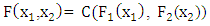 | (1) |
For every  where
where  represents the extended real line. Conversely, if
  is a copula and
  are distribution functions then the function
  defined a joint distribution function with margins
  The parametric copula approach ensures a high level of flexibility for modeling, because the dependence structure can be separated from the margins, through the function
  with an underlying parameter
  which governs the intensity of the dependence.In the case that the bivariate distribution has a density
  , and this is available, we have
 | (2) |
where  is the copula density and it should be approximated in most cases.In general, a natural and very useful way to describe a smooth function on the interval (0, 1) is to apply the orthonormal system of Legendre polynomials. This leads to a function
  on (0, 1) as
 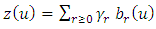 | (3) |
where  is the
  Legendre polynomial on (0, 1) and
  is the
  Fourier coefficient, such that
 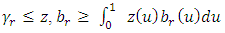 | (4) |
For example, the Legendre polynomials  are given by
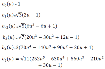 | (5) |
In the next section, it is seen that by using Legendre Polynomials a copula density function (given a known starting copula density function) is approximated.
3. Exponential Families
The exponential families are well-known families of parametric models that are used for approximating copula density function. If  is the starting copula density function, the desired copula density is then approximated by
 | (6) |
where  and
and  are Legendre polynomials,
  is the vector of parameters and
  is a normalizing function given by
 | (7) |
Obviously, increasing the number of parameters yields to model with more complexity, so in order to balance between complexity and the number of parameters, dimension  is determined. Note that
  may contain unknown parameters, which should be estimated as well. Equation (2) shows that
  is approximated by a linear combination of the functions
  minus a normalizing factor
  (to make its integral equal to 1). Exponential families ensure automatically that we get densities such that
  belongs to the natural parameter space
 | (8) |
The criteria for choosing the best approximation might be the Kullback Leibler information,  given by
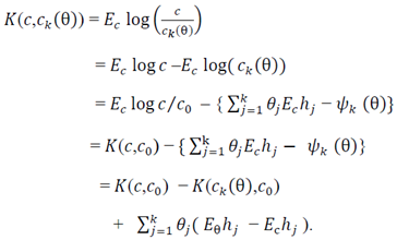 | (9) |
It is seen that minimizing  is equivalent to maximizing
  , which gives the asymptotic version of the maximum likelihood estimator. So, asymptotically the maximum likelihood estimator chooses that member
  of the exponential family which is closest to the true density
  in terms of Kullback Leibler information criteria.Kallenberg (2008) showed that
  is the projection of
  into the exponential family with base
  , because
  | (10) |
 | (11) |
Where  is a unique point such thatHence
  as the model error, is reduced to
  with a reduction equal to
  Another extra reduction from taking a higher dimension, when going from
  is occurred by an amount
 For the exponential family, the better fit means the smaller model error and the higher dimension or the more parameters have to be estimated. Since parameters estimation in the exponential family is difficult, the idea of contamination family is developed.
4. Contamination Families
As mentioned in Kallenberg (2009), just like the exponential family, the starting point is a copula density  and
and  is approximated by a linear combination of the functions
  hence
hence | (12) |
where  are Fourier coefficients as follows
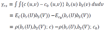 | (13) |
These coefficients depend on the unknown copula density function  that if it is replaced with empirical copula mass function
  then
then  can be estimated as
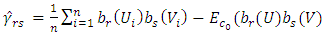 | (14) |
Again when the starting copula density function  belongs to a parametric family, its parameters should be estimated, then we have
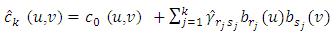 | (15) |
Kallenberg (2009) showed that by considering the term 
 as the model error given by
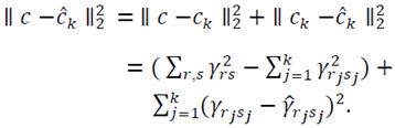 | (16) |
where  By equation (16) it can be seen that Total Error is decomposed by Model Error and Stochastic Error, Total Error = Model Error + Stochastic ErrorThe model error
  expresses how good the contamination family approximates the true density
  and the stochastic error
  is due to estimation.
4.1. Model Selection
In order to obtain parameter estimations in contamination family, the best dimension should be chosen. Suppose  be the largest dimension of r and s with
  observations, then we have
 | (17) |
For the selection rule, taking all the coefficients  for
for  yields a large estimation error, so we consider only the largest Fourier coefficients and ignore the rest. Therefore, the estimator from (17), is replaced by restricting to the
  largest among
  with
with  yielding
 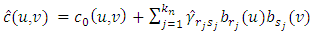 | (18) |
With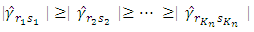 | (19) |
Random variables  and
and  depend on the data, and they are not chosen in advance. So how large should we take
  The optimal choice depends on
  but
but  is unknown, hence a data-driven selection of the dimension is taken.From (9), the model error for
  is
is 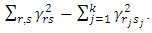 Hence,
  should grow sufficiently fast in order to take a higher dimension. For that purpose a penalty is introduced, classical penalties are for example
  (Schwarz’s rule) or
  (Akaike’s criterion). It may be better to take a larger penalty, taking into account the variance of
  .Kallenberg (2009), introduced a penalty as
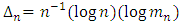 | (20) |
And the selection rule as: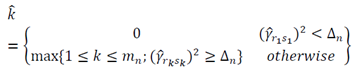 | (21) |
The estimated copula density now becomes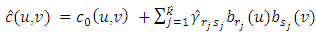 | (22) |
5. Copula Density Estimation for Iranian Household Income and Expenditure
The 2015  survey was carried out by a sample of 18839 households in urban areas and 19340 households in rural areas. The survey target population includes all private and collective settled households in urban and rural areas.
  three-stage cluster sampling method with strata is used in the survey. At the first stage, the census areas are classified and selected. At the second stage, the urban and rural blocks are selected and the selection of sample households is done at the third stage. The number of samples is optimized to estimate average annual income and expenditure of the sample household based on the aim of the survey. In this section, the model selection method is used to estimate copula density for Iranian Household Income and Expenditure
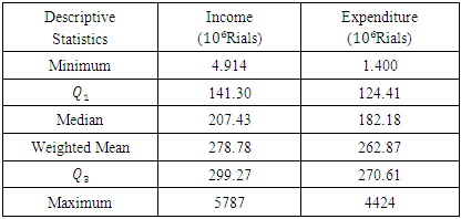
  Income and Expenditure descriptive statistics of urban and rural household are shown in Tables 1 and 2, respectively.
Table 1. Descriptive statistics for Income and Expenditure data of Urban household
 |
| |
|
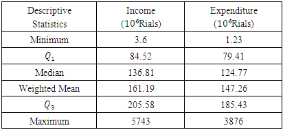
Table 2. Descriptive statistics for Income and Expenditure data of Rural household
 |
| |
|
5.1. IHIE Copula Density Estimation with Contamination Families
By using empirical distributions as marginal distribution estimations for both variables as | (23) |
Now the problem is to estimate the unknown copula function. In order to use a few largest Fourier coefficients, the absolute value of the Fourier coefficients are arranged from largest to smallest and compare with 
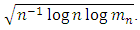 By using the sample size of each data set
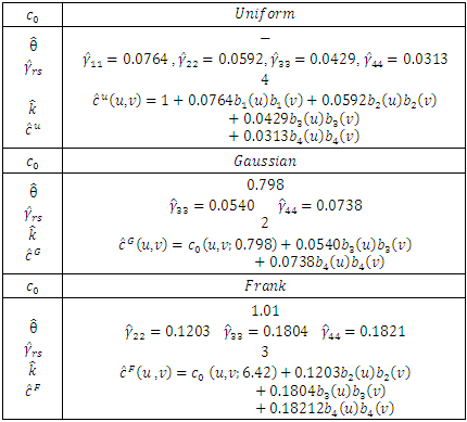
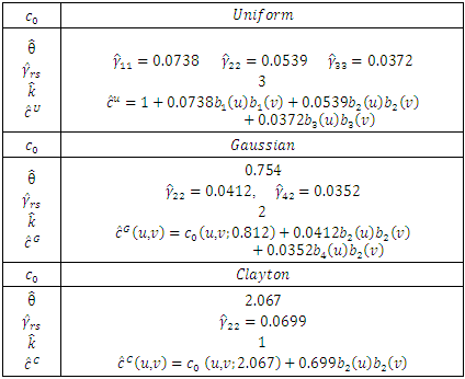
  is calculated, then according to the chosen algorithm of Fourier coefficients, these coefficients are obtained. With several start copula densities (Uniform, Gaussian, Clayton and, Frank), as it is shown in Tables 3 and 4, we have several estimations of copula density for rural and urban data sets.
Table 3. Results for Urban Data
 |
| |
|
Table 4. Results for Rural Data
 |
| |
|
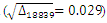
For Urban data the sample size is  , with
  calculation gives that
 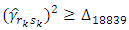 for
for 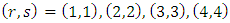 , so
, so  and
and 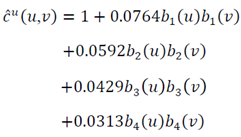 | (24) |
With the Gaussian copula density as the start point, calculations give 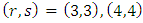 , so
, so  and
and 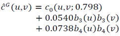 | (25) |
For the start with Frank copula density calculations give 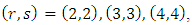 so
so  and
and 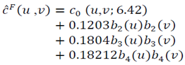 | (26) |
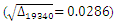
For Rural data the sample size is  with
with  calculation gives that
  for
for  so
so  and
and 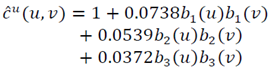 | (27) |
With the Gaussian copula density as a start point, calculations give  so
so  and
and 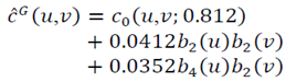 | (28) |
For the start with Clayton copula density calculations give  , so
, so  and
and  | (29) |
It should be noted that without using this method (selection method) among known copula densities, Frank copula and Clayton copula are the appropriate copulas for Urban and Rural data respectively, here these copulas can be chosen as starting points.
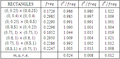
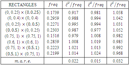
5.2. Investigating Performance of the Estimated Copula Function
To check the performance of the estimated copula densities, frequency of data is compared with the estimated probabilities, based on mean absolute relative error 
 on the same symmetric rectangles
  and asymmetric rectangles
 and also the corresponding upper tail rectangles.It can be seen from Table 5 for Urban data copula density function
  with Gaussian copula as a starting point has the least
  Also Table 6 shows that for Rural data copula density function
  with Gaussian copula as the starting point has the least
Table 5. The frequencies and approximations on different rectangles for Urban data
 |
| |
|
Table 6. The frequencies and approximations on different rectangles for Rural data
 |
| |
|
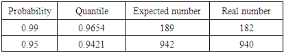
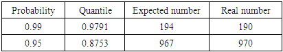
For more investigating of this new method, we considered the 99% (95%) quantile  based on
  (for both datasets) and the actual number of data points
  outside the rectangle
  with the expected number which is
  or
or  was compared. The results are shown in Tables 7 and 8. In both tables, the expected numbers and the real numbers are close to each other.
Table 7. The 0.99 and 0.95 estimated and real quantiles for Urban data
 |
| |
|
Table 8. The 0.99 and 0.95 estimated and real quantiles for Rural data
 |
| |
|
6. Conclusions
In this paper in order to approximate copula density function for two variables, Income and Expenditure, of Iranian household, contamination families and selection models methods have been used. In this approach, a sequence of parametric copulas has been considered and in a few numbers of steps, accurate approximations for copula densities are obtained. By using the selection model method, the model complexity and number of model parameters have been balanced. It was shown that the best approximations for copula density function are the ones that are based on Gaussian starting copula. Also by using m.a.r.e. as a criterion, it has been shown that for both cases approximation with Gaussian copula as the starting point has the least mean absolute relative error.
References
| [1] | Biau, G., Wegkamp, M., 2005. A Note on minimum distance estimation of copula densities. Statistics probability Letters 73, 105-114. |
| [2] | Emberchts, P., Lindskog, F., McNeil, A., 2003. Modelling dependence with copulas and applications to risk managements. Rachev, S.T. (Ed.), Handbook of Heavy Tailed Distributions in Finance. Elsevier, Amsterdam, 329-384. |
| [3] | Kallenberg, W.C.M., 2008. Modelling Dependence. Insurance: Mathematics and Economics, 2008, vol. 42, issue 1, 127-146. |
| [4] | Kallenberg, W.C.M. 2009. Estimating copula densities, using model selection techniques. Journal of Insurance: Mathematics and Economics 45 209-223. |
| [5] | McNeil, A., Frey, R., Emberchts, P., 2005. Quantitative Risk Management: Concepts, Techniques and Tools. Princeton University Press, Princeton. |
| [6] | Nelsen, R.B., 1999. An Introduction to Copulas. Lecture Notes in Statistics, 139. Springer Verlag, New York. |
| [7] | Sklar, A., 1959. Fonctions de repartition a n dimensions et leurs marges. Punl. Inst. Statist. Univ. Paris 8 229-231. 10. |
| [8] | Sklar, A., 1996. Random variables, distribution functions, and copulas- a personal look backward and forward. In Distributions with Fixed Marginals and Related Topics (L. Ruschendorf, B. Schweizer and M.D. Taylor, eds). 1-14, Lecture notes monograph series 28, Institute of Mathematical 2 Statistics, Hayward, CA. |

 Abstract
 Reference
 Full-Text PDF
 Full-text HTML