1. Introduction

The recent development in the field of cryptocurrency is receiving significant attention as it has become a significant means of making day to day business transactions. It is based on a fundamentally new technology, designed to work as a medium of exchange that uses cryptography to control its creation and management, rather than relying on central authorities [1]. Hence, its potential of which is not fully understood [2].

The most traded currency of the cryptocurrencies, Bitcoin, over the years has undergone rapid growth to become a significant currency both on and offline to the extent that some businesses has begun accepting Bitcoin in addition to traditional currencies. In the field of investment, the recent rise in the value of Bitcoin has led most investors to consider it as an investment opportunity, although several regulatory agencies have issued investor alerts about it.

Although, Bitcoin has been criticized for its use in illegal transactions, its high electricity consumption, price volatility, thefts from exchanges and the possibility that it is an economic bubble [3], its legal status varies substantially from country to country. Whereas many countries do not make the usage of bitcoin itself illegal, its status as money (or a commodity) varies with differing regulatory implications, thus, becoming a source of worry for investors and therefore needs due attention.

In the field of finance, one way to understand the dynamics of such volatile phenomenon is to investigate its returns and assess how investors and the markets value its prospects. In modelling such volatilities, a fundamental methodology is to measure potential losses of investment. Thus, the concept of Value at Risk (VaR), has become a widespread measure of market risk. However, the estimation of VaR requires the use of the Auto Regressive Conditional Heteroscedasticity (ARCH) model by [4], later generalized independently by [5] and [6] into the symmetric Generalized ARCH (GARCH). A thorough survey by [7] finds that GARCH generally dominates ARCH.

Today, several extensions of the traditional symmetric GARCH (p,q) model have been introduced to increase the flexibility of the original GARCH model such as asymmetric GARCH model which consist of the exponential GARCH (EGARCH), GJR-GARCH of [8], and the threshold GARCH (TGARCH) of [9]. These asymmetric GARCH models capture the characteristic of volatility and are today the most popular way of parameterizing this dependence as they tend to outperform the original GARCH by incorporating leverage effects [10].

In literature, various studies in attempt to improve volatility forecasting using GARCH introduces various error distribution ([11]; [12]; [13]). Though, several arguments have been made regarding the superiority among the error distributions, this study employs the three of the frequently used, namely: the Normal distribution (NORM), Student-t (STD), Generalized Error Distribution (GED). The main reason for choosing these types of error distributions is to consider the skewness, excess kurtosis and heavy-tails of return distributions.

Hence, this study seeks to model the volatility and Value at Risk of the daily returns of Bitcoins using symmetric and asymmetric GARCH models, given three different assumptions of the error distribution.

2. Material and Methods Used

2.1. Scope

Historical data on the daily prices of bitcoin online was taken from CoinMarketCap website (www.coinmarketcap.com/currencies/bitcoin/historical-data). The data spans from January 1, 2017 to September 12, 2018 totaling 620 observations. The daily closing prices was used in this paper.

2.2. Methods

The daily closing prices were changed to log returns given by Equation (1);

(1)

where is the logarithmic return at time is the current closing price at time t and is the previous closing price.

2.2.1. Jarque-Bera Test

Jarque-Bera test is a goodness-of-fit test which examines if the sample data have kurtosis and skewness similar to a normal distribution. The test is given by Equation (2);

(2)

where S and K are the skewness and kurtosis respectively. The JB test is done under the null hypothesis, H₀: normality, against the alternate, H₁: non-normality. If the sample data comes from a normal distribution JB should, asymptotically, have a chi-squared distribution with two degrees of freedom.

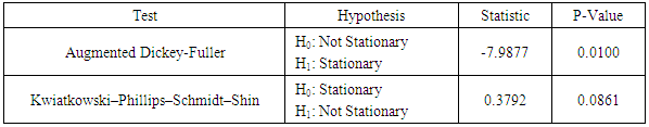
2.2.2. Unit Root Test: ADF Test

The Augmented Dickey-Fuller (ADF) test was used to determine whether the individual series studied have unit root or were covariance stationary. This method was proposed by [14] as an upgraded form of Dickey-Fuller Test. The unit root test is done under the null hypothesis (non-stationary) against the alternate (covariance stationary). Where is the characteristic root of an AR polynomial. The ADF test statistic is given by Equation (3);

(3)

where is a vector of deterministic terms (constant, trend etc.). The plagged difference terms, , are used to approximate the mean equation structure of the errors, , and the value of p is set so that the error, is serially uncorrelated.

Contrary to most unit root test, like ADF, the absence of a unit root is not a proof of stationarity, but by design, of trend-stationarity. This is being addressed by the Kwiatkowski-Phillips-Schmidt-Shin (KPSS) test developed by [15]. KPSS is defined by Equation (4)

(4)

where , is the residual of a regression of on and is a consistent estimate of the long-run variance of using .

2.2.3. The Mean Equation

It is imperative to specify an appropriate mean equation in modelling volatility. Following [16], this paper used the mean equation given by Equation (5);

(5)

where is the returns at time, and are constants and the innovation respectively.

2.2.4. Univariate GARCH Models

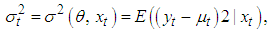
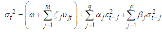
The returns of a financial asset largely depend on its volatility. In order to model such a phenomenon, the ARCH and then GARCH models by [4] and [5], respectively, needs to be considered. In GARCH models, the density function is usually written in terms of the location and scale parameters, with normalization vector given by Equation (6)

(6)

where the conditional mean is given by Equation (7)

(7)

and the conditional variance is expressed as Equation (8),

(8)

The rest of this section discusses the various forms and extensions of GARCH implemented in the study, whiles Section 2.2.5 focusses on the distributions implemented, as well as their standardization for use in GARCH processes.

The Standard GARCH Model (SGARCH)

The standard GARCH model developed by [5] is given by Equation (9):

(9)

where denotes the conditional variance, the intercept and the residuals from the mean filtration process. The GARCH order is defined by (q, p) (ARCH, GARCH). One of the key features of the observed behavior of financial data which GARCH models capture is volatility clustering which may be quantified in the persistence parameter, , defined as Equation (10)

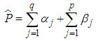(10)

Related to persistence parameter (), is the half-life (H), defined as the number of days it takes for half of the expected reversion back towards to occur. H is expressed as Equation (11)

(11)

The Threshold GARCH Model (TGARCH)

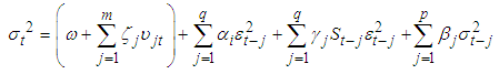This model was proposed by [9]. It is a re-specification of the GARCH model with an additional term to account for asymmetry (leverage effect). The general specification of the TGARCH (p, q) model is given by Equation (12);

(12)

where

From the model, depending on whether is above or below the threshold value of zero, can have different effects on the conditional variance . The persistence of the model is given by Equation (13)

(13)

where is the expected value of the standardized residuals below zero, and the half-life H is estimated using Equation (11).

2.2.5. Distributional Assumptions of Error Term

In GARCH model specification, it is more appropriate to consider the choice on the distributional assumption of the error term. This study assumed three distributional assumptions; Normal distribution (NORM), Student-t distribution (STD) and the Generalized Error Distribution (GED) in order to account for fat tails that are common in most financial data.

Normal Distribution (NORM)

For the models to fully function, the error term must have zero mean. That is where the error term in this case is normally distributed with zero mean and variance one. The density function for the Normal distribution is given by Equation (14)

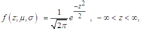(14)

where constitute the mean and is the standard deviation.

Student-t Distribution (STD)

The fatter tails, frequently observed in financial time series, are allowed for in the Student’s t distribution assumed by [17] which is given by the density function shown as Equation (15)

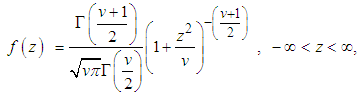(15)

where denotes the number of degrees of freedom and denotes the Gamma function.

Generalized Error Distribution (GED)

[11] proposed the use of the GED in order to account for fat-tails observed commonly in financial time series. It is given by Equation (16);

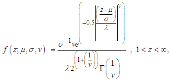(16)

is the degrees of freedom or tail-thickness parameter. If , the GED yields the normal distribution. If , the density function has thicker tails than the normal density function, whereas for it has thinner tails.

2.2.6. Model Selection Criterion

Two information criteria were used for model selection in this study. They are Akaike Information Criteria (AIC) and the Bayesian Information Criterion (BIC). AIC and BIC are defined as Equations (17) and (18) respectively:

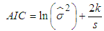(17)

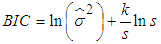(18)

where is the variance of the residuals, s is the sample size, k is the total number of parameters. For a GARCH (p,q) model, . The best model is the model that has least AIC and BIC values.

2.2.7. Model Diagnostics

It is very essential to perform a diagnostic check on the model after determining the best model and its corresponding distribution for the error term to establish whether the model and distribution are correctly specified. This study employs the Ljung-Box and Lagrange Multiplier (LM) tests to test for the presence of autocorrelation and ARCH effects respectively. The presence of autocorrelation and ARCH effects for the residuals of both the mean model and the volatility models will be tested using these two diagnostics.

Univariate Ljung-Box Test

The Ljung-Box Test is used to test whether there exist autocorrelations in the residuals of a model. The statistic is given by Equation (19);

(19)

where is the residual sample autocorrelation at lag i, s is the size of the series, k is the number of time lags included in the test. has an approximately chi-square distribution with k degree of freedom.

Testing for ARCH Effects

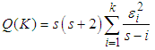
In applying GARCH methodology it is imperative to examine the residuals for any evidence of ARCH effects. The Lagrange Multiplier (LM) and the Ljung-Box statistic tests are used to test the ARCH effect in the residuals of a model by letting the lag autocorrelation of the squared residuals to be , the Ljung-Box statistic is given by Equation (20);

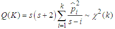(20)

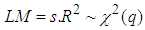The statistic of the LM test is given by Equation (21);

(21)

where q is the number of restrictions placed on the model, s is the size of the series and forms the regression.

2.2.8. Evaluation of Volatility Forecast

To evaluate the forecasting performance of the GARCH models, this study made use of two error measures; Mean Absolute Error (MAE) and the Mean Square Error (MSE). The MAE and MSE are defined as Equations (22) and (23) respectively

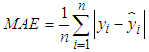(22)

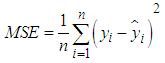(23)

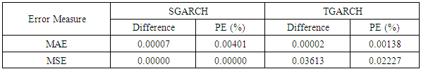
where is the observed value; is the fitted value; n is the sample size.

In situations where the best fitted models do not provide the best volatility forecasts in terms of the values of MSE and MAE, the Percent Error (PE) of MSE/MAE for each underlying case is evaluated. This will help investigate the difference of the values of MSE/MAE given by the best fitted model and the best performance model. PE is defined as Equation (24)

(24)

where A denotes MAE/MSE given by the best fitted model and B denotes MAE/MSE given by best performance model.

2.2.9. Value-at-Risk

VaR can be viewed as a gauge that summarizes the worst loss over a target horizon that will not be exceeded with a given level of confidence [18]. More formally, is expressed as Equation (25)

(25)

where L is the loss on a given day and is the significance level. VaR is therefore a quantile in the distribution of profit and loss that is expected to be exceeded only with a certain probability, which is given Equation (26)

(26)

Throughout this study, the VaR were observed at 1% significance level. VaR would be computed using the conditional volatility of returns multiplied by the quantile of a given probability distribution.

2.2.10. Backtesting VaR

Finding suitable forecast models for VaR estimates requires a method for evaluating the predictions ex-post. The VaR estimates in this study would be evaluated using two tests: an unconditional and a conditional test of coverage originally developed by [19].

Thus, daily returns would be labelled according to Equation (27) in order to define whether the daily return exceeded the VaR estimate or not. The indicator variable is constructed as shown in Equation (27)

(27)

where 1 indicates a violation and 0 indicates a return less than the VaR. The violations are thereafter summed and divided by the total number of out-of-sample VaR estimates with the intention of obtaining the empirical size.

Christoffersen’s Joint Test of Unconditional Coverage and Independence

The advantage with the Christoffersen test of independence is its deference to the conditionality in the volatility forecasts. This is given by Equation (28)

(28)

where is the number of observations with the value i followed by j for and is the corresponding probabilities. under the null hypothesis which states that the violations are independently distributed. Hence, a rejection of the null hypothesis infers that the violations are clustered and consequently not independent.

3. Results and Discussions

3.1. Preliminary Analysis of Data

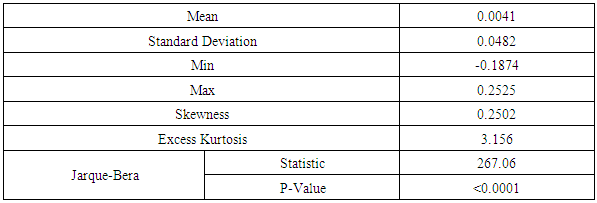
The descriptive statistics of return of Bitcoins is presented in Table 1. As observed, the average return within the study period was 0.0041. The returns showed a positive skewness with indication of leptokurtic (Excess Kurtosis > 3) depicting increased in probability at the higher quantiles (heavy and longer right tails). Also, the return series does not follow a normal distribution since normality test for it is firmly rejected by the Jarque-Bera statistics (P-Value < 0.05).

Table 1. Descriptive Statistics of Returns

Figure 1(a) shows the pattern of daily returns of Bitcoin. As observed, the series displays a considerable level of variation indicating little evidence of seasonality. Also, the change in variations from day to day throughout the period indicates the existence of stationarity. This was confirmed by the Autocorrelation Function (ACF) and the Partial ACF (PACF) plots in Figures 1(b) and 1(c). They show a very fast decay which is typical of a stationary series. To validate this claim, the Augmented Dickey-Fuller (ADF), as well as the Kwiatkowski-Phillips-Schmidt-Shin (KPSS) test, were, therefore computed as shown in Table 2. As observed, the series under consideration is stationary (p-value of ADF < 0.05; p-value of KPSS > 0.05).

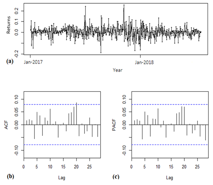Figure 1. Time Series Plot of Daily Returns of Bitcoins

Table 2. Stationarity Test

In volatility modelling, the first step is selection of suitable ARMA (p, q) model for the daily return of Bitcoins. By observing the ACF and the PACF in Figure 1(b) and 1(c), a rough order of p and q could be acquired. But, in selecting the ‘best’ mean model for the subsequent volatility models, nine competing models were fitted, and the result shown in Table 3. The ‘best’ model is the model with the minimum Akaike or Bayesian Information Criteria (AIC or BIC). Thus, the ‘best’ model is ARMA (0,0). Regarding the diagnostic checking of the best mean model, the p-values from the Box-Ljung test in Table 4 indicates that the residuals of the model are uncorrelated (0.6971>0.05). However, the p-values from ARCH LM test and the Box-Ljung test of the squared residuals confirm the existence of ARCH effects in the mean model. This implies that the ARMA (0,0) model does not explain the times series efficiently; hence, an ARCH or GARCH model should be employed in modelling the return time series.

Table 3. Competing Mean Models and Information Criteria

Table 4. Selected Mean Model Diagnostics

3.2. GARCH Modelling

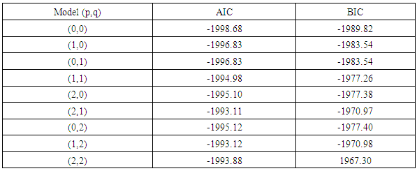
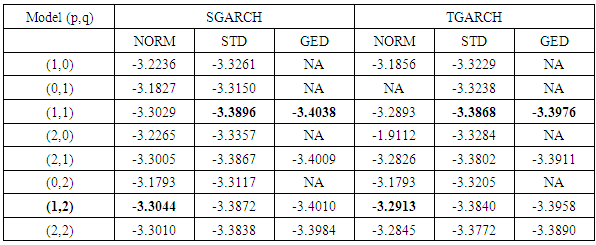
For the purpose of cross validation, the series is divided into two subsets. The first subset is called in-sample data set (full sample with 31-days/one month shorter, i.e. up to end of 11^th August 2018) used to build the GARCH models for underlying return series. The second subset, called out-sample data set (the remaining sample from 11^th August, 2018 to the end) is then used to validate the performance of volatility forecasting. Table 5 shows the Akaike Information Criteria (AIC) for the various combinations of the symmetric and asymmetric GARCH models computed under three (3) different error terms distributions.

Table 5. Summary of AIC of Computed GARCH Models

Under SGARCH models, SGARCH_GED (1, 1) had the least AIC value (-3.4038) which indicates that it was the best among the SGARCH models considered. With regards to the TGARCH models, TGARCH_GED (1, 1) had the least AIC value (-3.3976) which indicates that it is also the best among the TGARCH models considered. But, SGARCH_GED (1, 1) is considered to be the best model among all the models considered since it had the least AIC value. This indeed provides a compelling evidence made by Hansen and [20] and [21], that it is difficult to find a volatility model that outperforms the simple GARCH (1,1) basically due to its better numerical stability of estimation and parsimony. Although these best fitted models are expected to produce the most accurate forecast of volatility, [22] argues that the best fitted models based on AIC criterion are not necessarily able to provide the best forecast of volatility in terms of MSE and MAE.

3.2.1. Performance of Volatility Forecasting

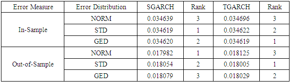
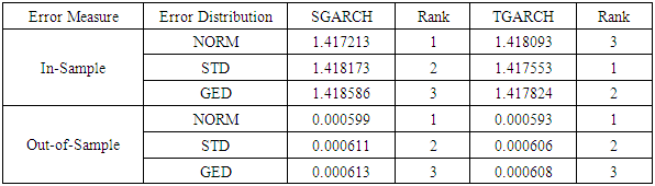
In order to ascertain the validity of [22] findings and determine the appropriate GARCH model, the volatility forecast performance from the in-sample and out-of-sample models were evaluated. Table 6 and 7 shows the evaluation of the best fitted GARCH models under each error distributions using two error measures (MAE and MSE).

Table 6. Mean Absolute Error (MAE) of Best Fitted GARCH Models

Table 7. Mean Square Error (MSE) of best Fitted GARCH Models

With regards to the Mean Absolute Error (MAE) estimates, the rankings from the in-sample analysis supports the claim that the best fitted models (TGARCH_GED (1,1) ranked 1^st) are indeed the best, except in the case of SGARCH_GED (1,1) where it ranked 2^nd. On the contrary, the rankings from the out-of-sample analysis does not support the claim of the best fitted models, thus, supports [22] findings.

With regards to the Mean Square Error (MSE) estimates, the rankings from both the in-sample and out-of-sample analysis in general does not supports the claim that the best fitted models (SGARCH_GED (1,1), and TGARCH_GED (1,1)) are the best. On the contrary, the rankings from both the in-sample and out-of-sample analysis favours the fitted GARCH models with normally distributed errors (NORM).

Error measures from both the in-sample and out-of-sample forecast (Tables 6 and 7) do not show a clear distinction of the best volatility models in terms of the values of MAE and MSE. Also, it supports the statement that, the best fitted model in terms of the AIC criterion does not necessarily provide the minimum values of MSE and MAE and hence, might not produce the best performance of forecasting volatility. This raises the question, how much difference between the best forecast and the forecast given by the best fitted model?

To investigate the difference of the MAE and MSE values given by the best fitted model and the best performance model, the Percent Error (PE) for each underlying case (GARCH-type model) is evaluated as shown in Table 8. As observed, majority of PE values are small and less than 0.03%. This implies that MAE and MSE values given by the best fitted model is not statistically different from that given by the best performance model. Thus, in practical situations, the best fitted model can still be used for volatility forecasting [23]. In this regard, the SGARCH_GED (1,1), with generalised error distribution terms is still noted to be the best fitted GARCH model to forecast the volatility of Bitcoin returns.

Table 8. Percentage Error of best Fitted Models and the best Performance Models

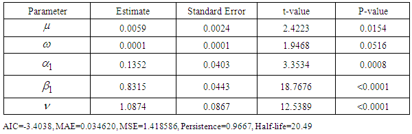
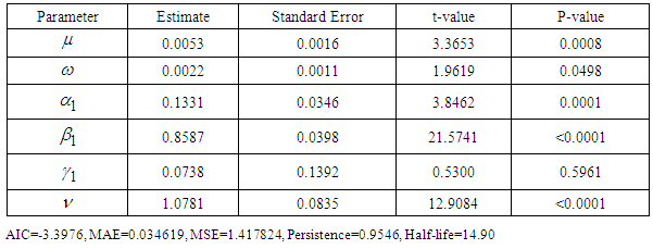
The parameter estimates of SGARCH_GED (1,1) and TGARCH_GED (1,1) are shown in Table 9 and 10 respectively. As observed, the p-values from the students t-test shows that most of the parameters in SGARCH_GED (1,1) and TGARCH_GED (1,1) are statistically significant at 5% level, which is an indication of how these parameters contribute significantly to the volatility models. For all fitted models, were significant (p-values<0.05) suggesting that volatility is persistent in the sense that the volatility of time is greatly affected by the volatility at time . Also, all the have their p-values less than 0.05 implying that the volatilities are less spiky since a shock at time (caused by an unusually high or low return) affects the volatility of time . With regards to the , only SGARCH_GED (1,1) has p-values greater than 0.05. The fact that is not different from zero means that the unconditional long run variance is zero. Also, the estimated volatility persistence is very high for all best fitted models and implies half-lives of shocks to volatility to SGARCH_GED (1,1) and TGARCH_GED (1,1) of 20 and 15 days, respectively. The shape parameter , showing the estimated degrees of freedom are slightly different from each other which implies that the density plot of all the best fitted models would look the same.

Table 9. Parameter Estimates of SGARCHGED (1,1)

Table 10. Parameter Estimates of TGARCH GED (1,1)

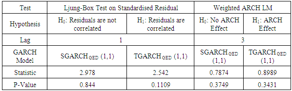
3.2.2. Model Diagnostics

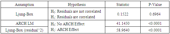
Table 11 shows the diagnostics on the best fitted GARCH models (SGARCH_GED (1,1) and TGARCH_GED (1,1)). As observed, the Ljung-Box test null hypothesis is not rejected at 5% significance level. This indicates that the standardized residuals are considered as white noise. Also, the weighted ARCH LM test indicates the presence of no ARCH effects in the models. These tests collectively suggest that the best fitted GARCH models are sufficient to correct the serial correlation of the return’s series in the conditional variance equation.

Table 11. Diagnostics of fitted GARCH Models

3.3. Returns of Bitcoins with 1% VaR Limits

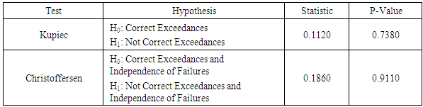
To validate the performance of the best fitted GARCH models, it is useful to perform a historical back-test to compare the estimated Value at Risk (VaR) with the actual return over the study period. If the return is less than the VaR in most cases, we have a VaR exceedance. In this study, a VaR exceedance is set to occur only in 1% of the cases, hence, the tests are evaluated on the 1% significance level. The start period of the back-test is set to 347 after the beginning of the series (i.e., January 2018). Also, The GARCH parameters are subsequently updated throughout the data set using rolling window estimation instead of being held constant over time. This is made in order to achieve flexibility in the parameters. The plot of the back-testing performance is shown in Figure 2.

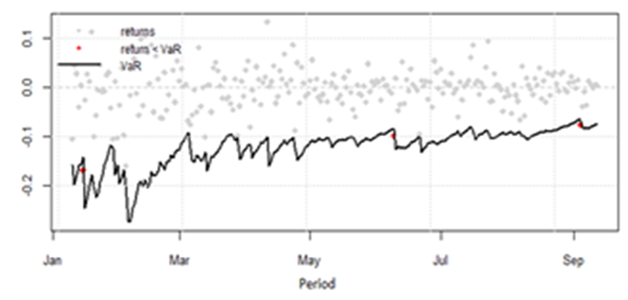Figure 2. 1% VaR Forecast at 1%

The VaR estimates produced by the volatility model are evaluated by Kupiec’s test [24] of unconditional coverage and Christoffersen’s test of independence. The tests are evaluated on the 1% significance level, hence the null hypothesis is rejected, and the model subsequently discarded, if the p-value is below one percent. All the fitted GARCH models (SGARCH_GED (1,1) and TGARCH_GED (1,1)) gave similar VaR Back-test results as shown in Table 12. From Table 12, despite the actual three (3) VaR exceedance versus an expected exceedance of 2.5, the null hypothesis that the exceedances are correct and independent is not rejected. This implies that a loss 1.2% is expected to be exceeded only 1% of the time.

Table 12. Coverage Test of Back-Testing

Overall, no model is clearly superior after evaluation through Kupiec’s unconditional coverage test and Christoffersen’s test of independence. Figure 3 shows the volatility forecast after the back testing. As observed, the volatility of Bitcoin returns in the first quarter of 2018 was relatively high but has been steadily decreasing with time. This could be as a result of the rejection of the first ever cryptocurrency exchange traded fund (ETF) by the US security exchange commission.

Expected Exceed=2.5, Actual VaR Exceed=3, Actual %=1.2%

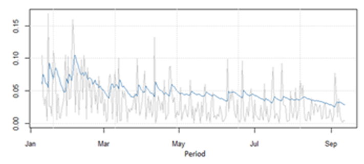Figure 3. Forecast of Volatility vs Daily Returns of Bitcoins (Absolute)

4. Conclusions

This paper modelled volatility and the Value at Risk (VaR) of daily returns of Bitcoins by conducting a comparative study in the forecast performance of symmetric and asymmetric GARCH models based on three different type of error distributions. The models include SGARCH and TGARCH. The performance of the models was evaluated using AIC, MAE and MSE. The results indicated that the SGARCH_GED (1,1) with generalised error distribution term was identified as the best fitted GARCH model computed based on the AIC criterion. This indeed provides a compelling evidence made that it is difficult to find a volatility model that outperforms the simple GARCH (1,1) basically due to its better numerical stability of estimation and parsimony. Though, these bests fitted model based on information loss (AIC) did not provide the best out-of-sample forecast, the error measures (MAE/MSE values) given by the best fitted models were insignificantly different from that given by the best forecast performance models. Since it is not practicable to identify the best performance model in practice, this study clearly demonstrates that it is reliable to use the best fitted model for volatility forecasting. Also, in order to further validate the performance of the best fitted model, it was subjected to a historical back-test using Value at Risk (VaR) at 1% significance level. Although, no model clearly emerged as superior, it was indicated that an average loss of 1.2% is expected to be exceeded only 1% of the time. Moreover, volatility forecast from the back testing was relatively high during the first quarter of 2018 but however begun decreasing steadily with time.