M. Tahmina Akter1, M. A. Mansur Chowdhury2
1Department of Mathematics, Chittagong University of Engineering & Technology, Chittagong, Bangladesh
2Jamal Nazrul Islam Research Center for Mathematical and Physical Sciences (JNIRCMPS), University of Chittagong, Chittagong, Bangladesh
Correspondence to: M. Tahmina Akter, Department of Mathematics, Chittagong University of Engineering & Technology, Chittagong, Bangladesh.
| Email: |  |
Copyright © 2019 The Author(s). Published by Scientific & Academic Publishing.
This work is licensed under the Creative Commons Attribution International License (CC BY).
http://creativecommons.org/licenses/by/4.0/

Abstract
An elegant and powerful technique is Homotopy Perturbation Method (HPM) to solve linearand nonlinear partial differential equations. Using the initial conditions this method provides an analytical or exact solutions. In this article, we shall be applied this method to get most accurate solution of a highly non-linear partial differential equation which is Reaction-Diffusion-Convection Problem. This article confirms the power, simplicity and efficiency of the method compared with the exact solution. This article also confirmed that this method is suitable method for solving any types of partial differential equations. A graphical representation of the result has been shown which provides the most accurate physical situation and accuracy of the solution. The HPM allows to find the solution of the nonlinear partial differential equations which will be calculated in the form of a series with easily computable components. From the calculation and its graphical representation it is clear that how the solution of the equation and its behavior depends on the initial conditions.
Keywords:
Homotopy perturbation method, Approximate solution, Exact solution, Nonlinear Reaction-Diffusion-Convection problem
Cite this paper: M. Tahmina Akter, M. A. Mansur Chowdhury, Homotopy Perturbation Method for Solving Highly Nonlinear Reaction-Diffusion-Convection Problem, American Journal of Mathematics and Statistics, Vol. 9 No. 3, 2019, pp. 136-141. doi: 10.5923/j.ajms.20190903.04.
1. Introduction
The homotopy perturbation method introduced first by the Chinese researcher Dr. Ji-Huan HE [1-5] for solving differential and integral equations, linear and nonlinear has been the subject of extensive analytical and numerical studies. Recently this method became popular and acceptable as an elegant tool in the hands of researchers because of its simplicity and give rise highly effective solutions of complicated problems in many diverse areas of science and technology. Many physical problems can be described by mathematical models that involve partial differential equations. In other words, a mathematical model is a simplified description of physical reality. The behavior of each model is governed by the input data for the particular problem: the boundary or initial conditions, the coefficient functions of the partial differential equation and the forcing function. This input data cause the solution of the model problem to possess highly localized properties in space in time or in both. Thus the investigation of the exact or approximate solution helps us to understand the means of these mathematical models and the real physical significance can be understood from the graphical representation of the solution. The aim of this article is to apply the Homotopy Perturbation Method (HPM) to obtain an approximate solution of a highly nonlinear partial differential equation -Reaction-Diffusion-Convection Problem with initial condition.The perturbation technique is one of the analytical methods to solve non-linear differential equations. This technique is widely used by engineers to solve some practical problems. Most often we obtain many interesting and important results by using this technique. However, the perturbation methods have their own limitations. Firstly, all perturbation techniques are based on small or large parameters so that at least one unknown must be expressed in a series of small parameters. But unfortunately, not every non-linear differential equation has such a small parameter. Mostly, the simplified linear equations have different properties from the original non-linear differential equation and sometimes some initial or boundary conditions are superfluous for the simplified linear equations. As a result, the corresponding initial approximations are perhaps far from exact. Clearly, these limitations of perturbations techniques come from the small parameter assumption. So it seems necessary to develop a kind of new non-linear analytical method which does not require small parameters at all. Ji- Huan He has described a non-linear analytical technique which does not require small parameters and thus can be applied to solve non-linear problems without small or large parameters. This technique is based on homotopy which is an important part of topology. Using one interesting property of homotopy, one can transform any non-linear problem into an infinite number of linear problems, no matter whether or not there exists a small or large parameter. The HPM is applied to Volterra’s integro-differetial equation [5], nonlinear oscillators [6], bifurcation of nonlinear problems [7], bifurcation of delay- differential equations [8], nonlinear wave equations [4] and to other fields [9-15]. The HPM yields a very rapid convergence of the solution series in most cases, usually only a few iterations leading to most accurate solutions. Thus He’s HPM is a universal one which can be solve many kinds of linear and nonlinear dynamical systems.This article is organized as follows. In section 2 illustrate the HPM introduced by He [1, 2]. In section 3 applied HPM to a highly nonlinear partial differential equation with initial condition for obtaining analytical solution which is most accurate. In section 4 the graphical representation of solution has also been displayed. We have also compared this analytical solution with the exact solution. Graphical and numerical results are discussed in section 5. Finally in section 6 the conclusion is provided.
2. Homotopy Perturbation Method
To achieve our goal, we have illustrated the basic idea of HPM to apply in a highly non-linear partial differential equations. Let us consider the following nonlinear differential equation of the form [1-15] | (1) |
with the boundary conditions: | (2) |
where  is a general differential operator,
  is a boundary operator,
  is a known analytical function and
  is the boundary of the domain
  . In general one can divide the operator into two parts: linear and non- linear. That means
 where
where  is a linear operator and
  is a non-linear operator.Hence, equation (1) can be rewritten as
  | (3) |
By the homotopy perturbation technique [1, 2], He construct a homotopy  which satisfies:
 | (4) |
Or | (5) |
where  is an embedding parameter,
  is an initial approximation which satisfies the boundary conditions. Obviously, from equations (4) and (5) we have:
  | (6) |
 | (7) |
The changing process of  from zero to unity is just that of
  from
from  to
to  . In topology, this is called deformation and
  and
and  are called homotopic. According to the HPM, we can first use the embedding parameter
  as a small parameter and assume that the solution of equations (6) and (7) can be written as a power series in
 | (8) |
Setting  results in the approximate solution of equation (1):
  | (9) |
The combination of the perturbation method and the homotopy method is called the homotopy perturbation method (HPM), which has eliminated the limitations of the traditional perturbation methods. On the other hand, this technique can have full advantage of the traditional perturbation techniques. The series (9) is convergent for most cases. However, the convergent rate depends on the nonlinear operator  : 1- The second derivative of
  with respect to
  must be small because the parameter may be relatively large, i.e.
  2- The norm of
  must be smaller than one so that the series converges.
3. Application
Let us consider the Reaction-Diffusion-Convection Problem [13] 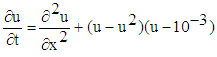 | (10) |
with the initial condition :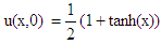 | (11) |
The exact solution of the problem (10) is given us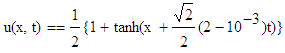 | (12) |
In order to solve equation (10) using homotopy- perturbation method, the homotopy perturbation technique can be constructed as follows: 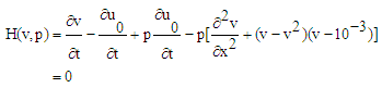 | (13) |
Suppose the solution of (10) has the form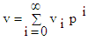 | (14) |
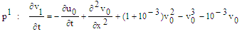
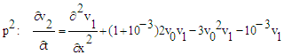
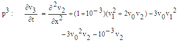
Substituting (14) into equation (13)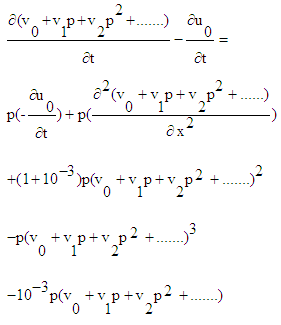 and comparing the coefficient of terms with identical powers of p, leads to:
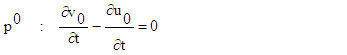 | (15) |
 | (16) |
 | (17) |
 | (18) |
and so on.Solving equation (15) and using the initial condition we get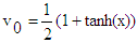 | (19) |
Again using the value of  and
and  we can find the solution of
  and similarly for other’s
  ’s.
’s. 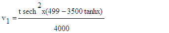 | (20) |
 | (21) |
and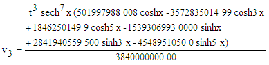 | (22) |
and so on.Therefore the approximate solution is given by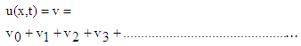 Hence
Hence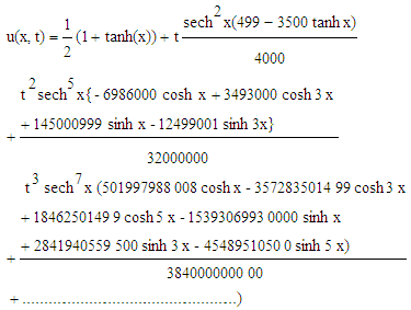 | (23) |
which is the approximate solution of equation (10).
4. Graphical Representation of above Equation
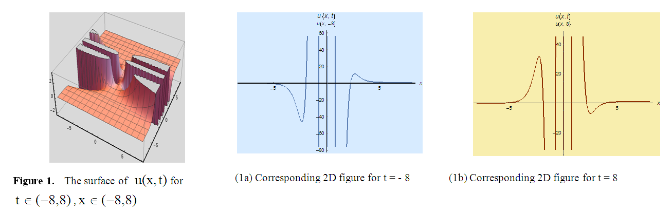 | Figure 1 |
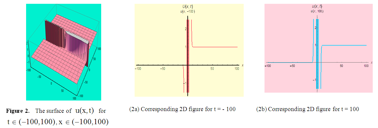 | Figure 2 |
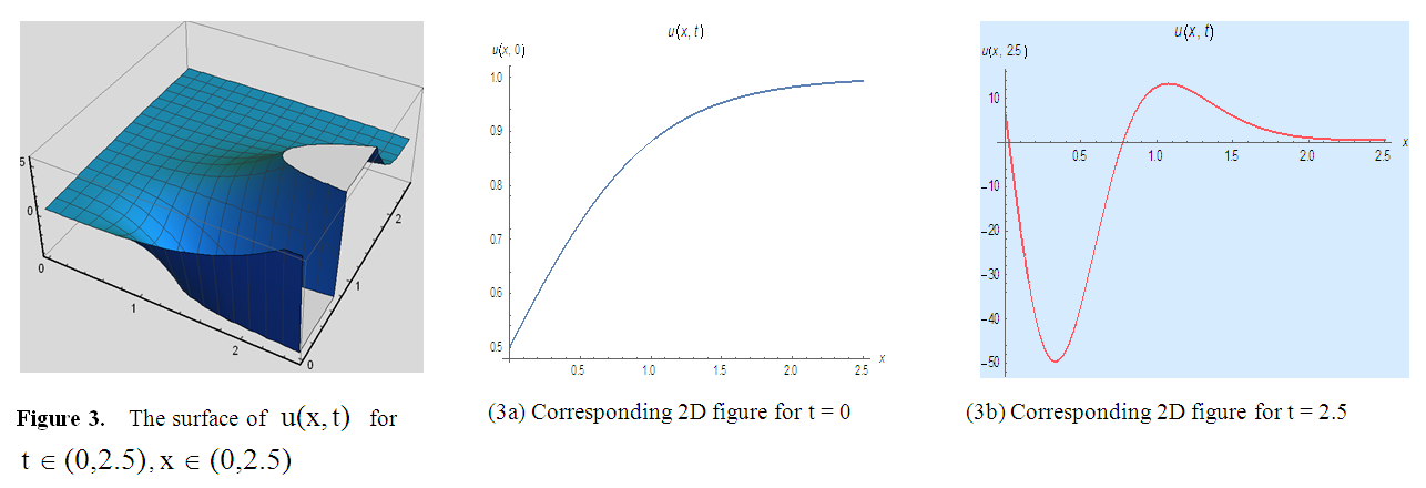 | Figure 3 |
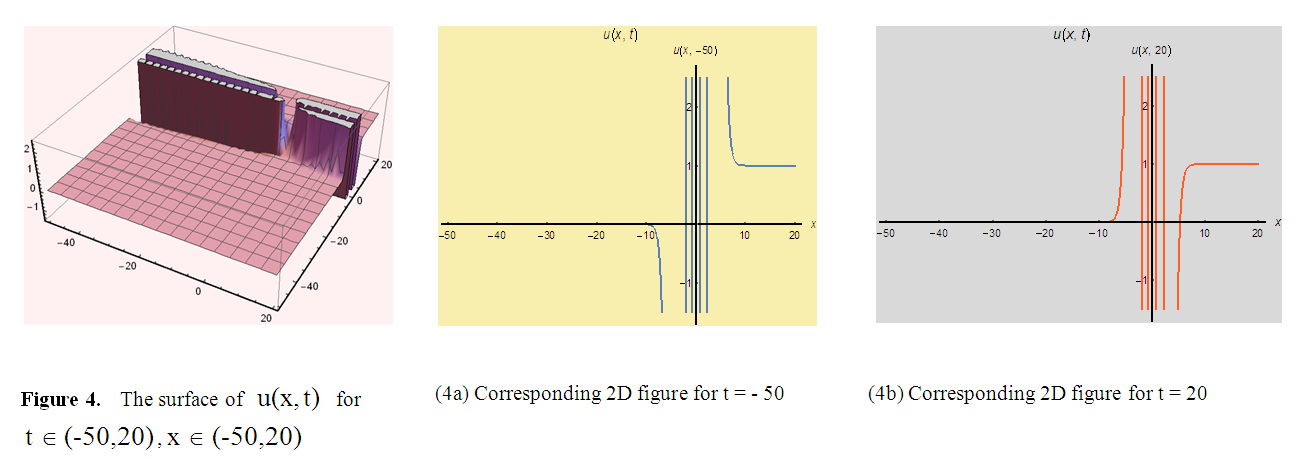 | Figure 4 |
 | Figure 5. The absolute error  and and  |
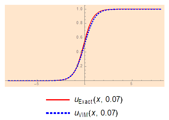 | Figure 6. The combined curves of Exact solution, the approximate solution (VIM) for a fixed value of  and for the range of the variable and for the range of the variable  respectively respectively |
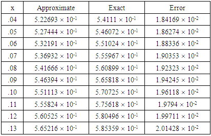
Table 1. Comparison of approximate and exact solution for the value of t = .03 of equation (23)
 |
| |
|
5. Result and Discussion of the Solution of Equation (10)
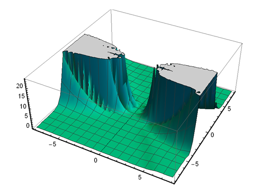
The computed results are presented graphically to observe the behaviour of the solution (23). The figures are drawn for different wide and short range of the variables x and t. From all figures we have seen that the curves are oscillated nearer to zero i.e. approximately in the range of  . The corresponding two dimensional graphs are seen by figures (1a), (1b), (2a), (2b), (3a), (3b) and (4a) (4b) for a fixed value of t specifically for the ending range of t and with the different ranges of variable x. In case of
  and
and  the absolute errors of the problem is displayed in figure 5. In figure 6 we have plotted the combined curves of exact solution, the approximate solution for a fixed value of
  and for
  respectively. From this figure it is clear that approximate solutions and exact solution are found in good agreement. From the table, we have seen the comparison result of approximate and exact solution for various
  and a fixed value
  . Here we observed that the errors are very significant. The results provides very strong evidence that is the homotopy perturbation technique easy to get approximate solution of nonlinear equation. It is to be note that four terms only were used in evaluating the approximate solutions.
6. Conclusions
He’s Homotopy perturbation method suggested in this article is an efficient method for obtaining the most accurate solution of a highly nonlinear partial differential equation with initial condition. Therefore, this method is a powerful mathematical technique to solve the wide classes of nonlinear partial differential equations in the form of analytical expressions. The HPM has got many important advantages and it does not require small parameters in the equation, so that the limitations of the traditional perturbations can be eliminated. Also the calculations in the HPM are simple and straightforward. The reliability of the method and the reduction in the size of the computational domain gives this method a wider applicability.
References
| [1] | J.H. He, “Homotopy perturbation technique”, Computer Methods in Applied Mechanics and Engineering, vol. 178, P-257-262, 1999. |
| [2] | J.H. He, “A coupling method of a homotopy technique and a perturbation technique for non-linear problems”, International Journal of Non-Linear Mechanic, vol. 35 (1) P-37-43, 2000. |
| [3] | J.H. He, “Homotopy perturbation method: A new nonlinear analytical technique”, Appllied Mathematics Computation, vol. 135 (1), P-73-79, 2003. |
| [4] | J.H. He,” Application of homotopy perturbation method to nonlinear wave Equations”, Chaos Solitons Fractals, vol. 26 (3), p-695-700, 2005. |
| [5] | M. El- Shahed, Moustafa, “Application of He’s Homotopy Perturvation Method to Volterra’s Integro- differential Equation, International Journal of Nonlinear Science of Simulation”, Vol. 6(2), p- 163-168, 2005. |
| [6] | J.H. He, “Asymptotology by homotopy perturbation method” , Appllied Mathematics Computation, vol. 156 (3), P-591-596, 2004. |
| [7] | J.H. He, “Homotopy perturbation method for bifurcation of nonlinear problems”, International Journal of Nonlinear Science of Simulation, vol. 6 (2), P-207-208, 2005. |
| [8] | He J. H, “Some Asymptotic Methods for Strongly Nonlinear Equations”, International Journal of Modern Physics B, vol. 20 p-1141–1199, 2006. |
| [9] | He J. H, “Recent development of homotopy perturbation method, Topology Methods in Nonlinear Analysis”, vol. 31, p-205-209, 2008. |
| [10] | M. Tahmina Akter, A. S. M. Moinuddin & M. A. Mansur Chowdhury, “Semi-Analytical Approach to Solve Non-linear Differential Equations and Their Graphical Representations, International Journal of Applied Mathematics & Statistical Sciences”, Vol. 3, Issue 1, p-35-56, 2014. |
| [11] | M. Tahmina Akter, M. A. Mansur Chowdhury, “Homotopy Perturbation Method for Solving Nonlinear Partial Differential Equations”, IOSR Journal of Mathematics, Volume 12 (5), PP 59-69, 2016. |
| [12] | M. Ghoreishi and A. I. B. Md. Ismail, “The Homotopy Perturbation Method (HPM) for Nonlinear Parabolic Equation with Nonlocal Boundary Conditions”, Applied Mathematical Sciences, Vol. 5( 3), p- 113 – 123, 2011. |
| [13] | Somjate Duangpithak and Montri Torvattanabun, “Variational Iteration Method for Solving Nonlinear Reation-Diffusion-Convection Problems”, Applied Mathematical Sciences, Vol. 6(17), p-843 – 849, 2012. |
| [14] | Ramesh Chand Mittal and Rakesh Kumar Jan, Numerical Solutions of nonlinear Fisher’s reaction-duffusion equation with modified cubic B-spline collocation method, Mathematical Sciences, Vol.7( 12), 2013. |
| [15] | Jafar Saberi-Nadjafi, Asghar Ghorbani, He’s homotopy perturbation method: An effective tool for solving nonlinear integral and integro-differential equations, Computers and Mathematics with Applications, Vol. 58, p-2379-2390, 2009. |

 Abstract
 Reference
 Full-Text PDF
 Full-text HTML