1. Introduction

In the process of developing the technology, many possible interesting adaptations became apparent: One of the most interesting directions was the use of the technology in the analysis of long DNA sequences. A benefit of the techniques was that it combined rigorous statistical analysis with modern computer power to quickly search for diagnostic patterns within long DNA sequences. Briefly, a DNA strand can be viewed as a long string of linked nucleotides. Each nucleotide is composed of a nitrogenous base, a five carbon sugar, and a phosphate group. There are four different bases that can be grouped by size, the pyrimidines, thymine (T) and cytosine (C), and the purines, adenine (A) and guanine (G). The nucleotides are linked together by a backbone of alternating sugar and phosphate groups with the carbon of one sugar linked to the carbon of the next, giving the string direction. DNA molecules occur naturally as a double helix composed of polynucleotide strands with the bases facing inward. The two strands are complementary, so it is sufficient to represent a DNA molecule by a sequence of bases on a single strand; refer to Fig. 1. Thus, a strand of DNA can be represented as a sequence of letters, termed base pairs (bp), from the finite alphabet.1 The order of the nucleotides contains the genetic information specific to the organism. Expression of information stored in these molecules is a complex multistage process. One important task is to translate the information stored in the protein-coding sequences (CDS) of the DNA (Polovinkina et al. (2016)).

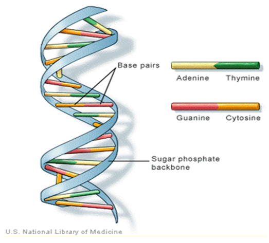Figure 1. The general structure of DNA and its bases

A common problem in analyzing long DNA sequence data is in identifying CDS that are dispersed throughout the sequence and separated by regions of noncoding (which makes up most of the DNA). Another problem of interest that we will address here is that of matching two DNA sequences, say and . The background behind the problem is discussed in detail in the study by Waterman and Vingron (1994). For example, every new DNA or protein sequence is compared with one or more sequence databases to find similar or homologous sequences that have already been studied, and there are numerous examples of important discoveries resulting from these database searches.

One naive approach for exploring the nature of a DNA sequence is to assign numerical values (or scales) to the nucleotides and then proceed with standard time series methods. It is clear, however, that the analysis will depend on the particular assignment of numerical values. Consider the artificial sequence ACGTACGTACGT. . . Then, setting A = G = 0 and C = T = 1, yields the numerical sequence 010101010101. . . , or one cycle every two base pairs (i.e., a frequency of oscillation of Cycle/bp, or a period of oscillation of length bp=cycle). Another interesting scaling is A = 1, C = 2, G = 3, and T = 4, which results in the sequence 123412341234. . . , or one cycle every four bp . In this example, both scalings of the nucleotides are interesting and bring out different properties of the sequence. It is clear, then, that one does not want to focus on only one scaling. Instead, the focus should be on finding all possible scalings that bring our interesting features of the data. Rather than choose values arbitrarily, the spectral envelope approach selects scales that help emphasize any periodic feature that exists in a DNA sequence of virtually any length in a quick and automated fashion. In addition, the technique can determine whether a sequence is merely a random assignment of letters (Polovinkina et al. (2016)).

Fourier analysis has been applied successfully in DNA analysis; McLachlan and Stewart (1976) and Eisenberg et al. (1994) studied the periodicity in proteins using Fourier analysis.

Stoffer et al. (1993) proposed the spectral envelope as a general technique for analyzing categorical-valued time series in the frequency domain. The basic technique is similar to the methods established by Tavar´e and Giddings (1989) and Viari et al. (1990), however, there are some differences. The main difference is that the spectral envelope methodology is developed in a statistical setting to allow the investigator to distinguish between significant results and those results that can be attributed to chance.

The article authored by Marhon and Kremer 2011, partitions the identification of protein-coding regions into four discrete steps. Based on this partitioning, digital signal processing DSP techniques can be easily described and compared based on their unique implementations of the processing steps. They compared the approaches, and discussed strengths and weaknesses of each in the context of different applications. Their work provides an accessible introduction and comparative review of DSP methods for the identification of protein-coding regions. Additionally, by breaking down the approaches into four steps, they suggested new combinations that may be worthy of future studies. A new methodology for the analysis of DNA/RNA and protein sequences is presented by Bajic in 2000. It is based on a combined application of spectral analysis and artificial neural networks for extraction of common spectral characterization of a group of sequences that have the same or similar biological functions. The method does not rely on homology comparison and provides a novel insight into the inherent structural features of a functional group of biological sequences. The nature of the method allows possible applications to a number of relevant problems such as recognition of membership of a particular sequence to a specific functional group or localization of an unknown sequence of a specific functional group within a longer sequence. The results are of general nature and represent an attempt to introduce a new methodology to the field of biocomputing. Fourier transform infrared (FTIR) spectroscopy has been considered by Han et al. in 2018 as a powerful tool for analysing the characteristics of DNA sequence. This work investigated the key factors in FTIR spectroscopic analysis of DNA and explored the influence of FTIR acquisition parameters, including FTIR sampling techniques, pretreatment temperature, and sample concentration, on calf thymus DNA. The results showed that the FTIR sampling techniques had a significant influence on the spectral characteristics, spectral quality, and sampling efficiency. Ruiz et al. 2018 proposed a novel approach for performing cluster analysis of DNA sequences that is based on the use of Genomic signal processing GSP methods and the K-means algorithm. We also propose a visualization method that facilitates the easy inspection and analysis of the results and possible hidden behaviors. Our results support the feasibility of employing the proposed method to find and easily visualize interesting features of sets of DNA data. A novel clustering method is proposed by Hoang et al. in 2015 to classify genes and genomes. For a given DNA sequence, a binary indicator sequence of each nucleotide is constructed, and Discrete Fourier Transform is applied on these four sequences to attain respective power spectra. Mathematical moments are built from these spectra, and multidimensional vectors of real numbers are constructed from these moments. Cluster analysis is then performed in order to determine the evolutionary relationship between DNA sequences. The novelty of this method is that sequences with different lengths can be compared easily via the use of power spectra and moments. Experimental results on various datasets show that the proposed method provides an efficient tool to classify genes and genomes. It not only gives comparable results but also is remarkably faster than other multiple sequence alignment and alignment-free methods. One challenge of GSP is how to minimize the error of detection of the protein coding region in a specified DNA sequence with a minimum processing time. Since the type of numerical representation of a DNA sequence extremely affects the prediction accuracy and precision, by this study Mabrouk in 2017 aimed to compare different DNA numerical representations by measuring the sensitivity, specificity, correlation coefficient (CC) and the processing time for the protein coding region detection. The proposed technique based on digital filters was used to read-out the period 3 components and to eliminate the unwanted noise from DNA sequence. This method applied to 20 human genes demonstrated that the maximum accuracy and minimum processing time are for the 2-bit binary representation method comparing to the other used representation methods. Results suggest that using 2-bit binary representation method significantly enhanced the accuracy of detection and efficiency of the prediction of coding regions using digital filters. Identification and analysis of hidden features of coding and non-coding regions of DNA sequence is a challenging problem in the area of genomics. The objective of the paper authored by Roy and Barman in 2011 is to estimate and compare spectral content of coding and non-coding segments of DNA sequence both by Parametric and Nonparametric methods. Consequently an attempt has been made so that some hidden internal properties of the DNA sequence can be brought into light in order to identify coding regions from non-coding ones. In this approach the DNA sequence from various Homo Sapien genes have been identified for sample test and assigned numerical values based on weak-strong hydrogen bonding (WSHB) before application of digital signal analysis techniques. The statistical methodology applied for computation of Spectral content are simple and the Spectrum plots obtained show satisfactory results. Spectral analysis can be applied to study base-base correlation in DNA sequences. A key role is played by the mapping between nucleotides and real/complex numbers. In 2006, Galleani and Garello presented a new approach where the mapping is not kept fixed: it is allowed to vary aiming to minimize the spectrum entropy, thus detecting the main hidden periodicities. The new technique is first introduced and discussed through a number of case studies, then extended to encompass time-frequency analysis.

For analyzing periodicities in categorical valued time series, the concept of the spectral envelope was introduced by Stoffer et al., 1993 as a computationally simple and general statistical methodology for the harmonic analysis and scaling of non-numeric sequences. However, The spectral envelope methodology is computationally fast and simple because it is based on the fast Fourier transform and is nonparametric (i.e., it is model independent). This makes the methodology ideal for the analysis of long DNA sequences. Fourier analysis has been used in the analysis of correlated data (time series) since the turn of the century. Of fundamental interest in the use of Fourier techniques is the discovery of hidden periodicities or regularities in the data. Although Fourier analysis and related signal processing are well established in the physical sciences and engineering, they have only recently been applied in molecular biology. Since a DNA sequence can be regarded as a categorical-valued time series it is of interest to discover ways in which time series methodologies based on Fourier (or spectral) analysis can be applied to discover patterns in a long DNA sequence or similar patterns in two long sequences. Actually, the spectral envelope is an extension of spectral analysis when the data are categorical valued such as DNA sequences.

An algorithm for estimating the spectral envelope and the optimal scalings given a particular DNA sequence with alphabe , is as follows (Stoffer 2012).

1. Given a DNA sequence of length n, from the vectors ; namely, for 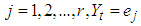if where is a vector with a 1 in the jth position as zeros elsewhere, and if .

2. Calculate the Fast Fourier Transform FFT of the data, .

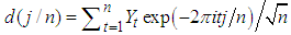Note that is a complex-valued vector. Calculate the periodogram,

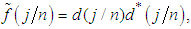for , and retain only the real part, say .

3. Smooth the real part of the periodogram as preferred to obtain , a consistent estimator of the real part of the spectral matrix.

4. Calculate the variance–covariance matrix of the data, 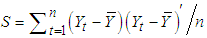, where is the sample mean of the data.

5. For each 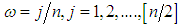, determine the largest eigenvalue and the corresponding eigenvector of the matrix

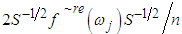6. The sample spectral envelope is the eigenvalue obtained in the previous step.

7. The optimal sample scaling is 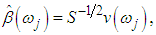where the eigenvector obtained in the previous step.

In this paper, we discussed the kernel density estimation for the first, second, third and fourth eigenvalues of variance covariance matrix of Fast Fourier Transform for numerical values representation of DNA sequences of five organisms, Human, E. coli, Rat, Wheat and Grasshopper. We computed an empirical values for the kernel density estimation for data series according to the following Kernels: Gaussian, Epanechnikov, Rectangular, Triangular, Biweight, Cosine, and Optcosine. To determine the valuable of our work, it should be noted that it is the first time that the variance covariance matrix eigenvalues of Fast Fourier Transform (FFT) for numerical values representation of DNA sequences, is used in an analysis like this and related analyzes.

2. Kernel Density Estimation

The problem of estimation of a probability density function f (x) is interesting for many reasons, among which are the possible applications in the field of discriminant analysis or the estimation of functions of the density. The parametric approach to density estimation assumes a functional form for the density and then estimates the unknown parameters using techniques such as the maximum likelihood estimation or Pearson system based on the estimation of the skewness and the Kurtosis (Oja (1981)). Unless the form of density is known a priori, assuming a functional form for a density very often leads to erroneous inference. It is clear that, nonparametric methods do not make any assumptions as to the form of the underlying density. Today, a rich basket of nonparametric density estimators (Kernel, orthogonal series, histogram, etc.) exists (Bowman and Azzalini (1997); Hall (1982); Silverman (1986)). On other words, the parametric methods assumes that the data is drawn from a known parametric family of distributions, for example a normal distribution but the nonparametric methods does not make this assumption. The main restriction of parametric methods is that they impose restrictions on the shapes that f can have (Lopez-Novoa et al. (2015)). This work focuses on kernel density estimators (KDE).

The kernel density estimator represents one of the important scientific subjects in spectrum theory. It is evident that, the kernel density estimator is a very useful nonparametric method and is very robust to the shape of distribution. An attractive feature of the kernel density estimator is that the resulting estimator can always be bimodal for an appropriate choice of bandwidth, which controls the smoothness of the estimator (Bae and Kim (2008)). Several techniques have been proposed for optimal bandwidth selection. The best known of these contain rules of thumb, oversmoothing, least squares cross-validation, direct plug-in methods, solve-the-equation plug-in method, and the smoothed bootstrap Jones, Marron and Sheather, (1996).

KDE is a common tool in many research areas, used for a variety of purposes, some of the relevant scientific literatures are as follows.

Andre´s Ferreyra et al. in (2001) used density estimates to forecast weather and other factors as part of a model for optimizing maize production. In the same field, it has been applied to evaluate the signature of climate change in the frequency of weather regimes (Corti et al., 1999). Furthermore, in the field of evolutionary computation, density estimation has been used to estimate a distribution of the problem variables in estimation of distribution algorithms (Bosman and Thierens, 2000).

Li et al. in (2007) suggested a nonparametric estimator of the correlation function for data, using kernel methods. They developed a pointwise asymptotic normal distribution for the suggested estimator, when the number of subjects is fixed and the number of vectors or functions within each subject goes to infinity. Based on the asymptotic theory, they suggested a weighted block bootstrapping method for making inferences about the correlation function, where the weights account for the inhomogeneity of the distribution of the times or locations. The method is applied to a data set from a colon carcinogenesis study, in which colonic crypts were sampled from a piece of colon segment from each of the rats in the experiment and the expression level of p27, an important cell cycle protein, was then measured for each cell within the sampled crypts.

Troudi et al. in (2008) suggested a faster procedure than that of the common plug-in method. The mean integrated square error (MISE) depends directly upon J(f) which is linked the second-order derivative of the pdf. They presented an analytical approximation of J(f), such that the pdf is estimated only once, at the end of iterations. Thus, these two kinds of algorithm are tested on different random variables having distributions known for their difficult estimation.

Bae and Kim in 2008 presented a kernel density estimation approach for the segmentation of the microarray spot. They estimated the density of n pixel intensities for a given target area by the kernel density estimation, and the resulting kernel density estimate gives bimodal density by appropriate choice of the smoothing parameter. They proposed two modes of the kernel density estimate for n pixel intensities as estimates of the foreground (mode with larger value) and the background (mode with smaller value) intensity, respectively.

Fan et al. in (2010) studied nonparametric estimation of genewise variance for microarray data. Microarray experiments are one of widely used technologies nowadays, allowing scientists to monitor thousands of gene expressions simultaneously. They presented a two-way nonparametric model, which is an extension of the famous Neyman-Scott model and is applicable beyond microarray data. The problem itself posed interesting challenges because the number of nuisance parameters is proportional to the sample size and it is not obvious how the variance function can be estimated when measurements are correlated. In such a high-dimensional nonparametric problem, they suggested two novel nonparametric estimators for genewise variance function and semiparametric estimators for measurement correlation, via solving a system of nonlinear equations. Their asymptotic normality is established. The finite sample property is demonstrated by simulation studies. The estimators also improve the power of the tests for detecting statistically differentially expressed genes.

Weyenberg et al. in (2014) suggested and implemented KDETREES, a non-parametric method for estimating distributions of phylogenetic trees, with the goal of identifying trees that are significantly different from the rest of the trees in the sample. This method compared favorably with a similar recently published method, featuring an improvement of one polynomial order of computational complexity (to quadratic in the number of trees analyzed), with simulation studies proposing only a small penalty to classification accuracy. Application of KDE TREES to a set of apicomplexa genes identified several unreliable sequence alignments that had escaped previous detection, as well as a gene independently reported as a possible case of horizontal gene transfer. They also analyzed a set of Epichlo€e genes, fungi symbiotic with grasses, successfully identifying a contrived instance of paralogy. An extensive list of application fields of KDE can be found in Sheather (2004).

Colbrook et al. in (2018) considered a new type of boundary constraint, in which the values of the estimator at the two boundary points are linked. They provided a kernel density estimator that successfully incorporates this linked boundary condition. This is studied via a nonsymmetric heat kernel which generates a series expansion in nonseparable generalised eigenfunctions of the spatial derivative operator. Despite the increased technical challenges, the model is proven to outperform the more familiar Gaussian kernel estimator, yet it inherits many desirable analytical properties of the latter KDE model.

The probability distribution of a random variable X is described through its probability density function (PDF) f. This function f gives a natural description of the distribution of X, and allows us to determine the probabilities associated with X using the relationship

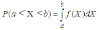Given several observed data points (samples) from a random variable X, with unknown density function f, density estimation is used to create an estimated density function from the observed data. Here, we use the non-parametric approach (KDE).

Furthermore, one of the most common techniques for density estimation of a continuous variable is the histogram, which is a representation of the frequencies of the data over discrete intervals (bins). It is widely used due to its simplicity, but it has several shortcomings, such as the lack of continuity. The KDE technique relies on assigning a kernel function K to each sample (observation in the dataset), and then summing all the kernels to obtain the estimate. In contrast to the histogram, KDE constructs a smooth probability density function, which may reflect more accurately the real distribution of the data. We now describe the KDE technique in more detail as follows (Lopez-Novoa et al. (2015)).

Let represent a random sample of size n from a random variable with density . Silverman in1986 defined the following kernel density estimate of f at the point by

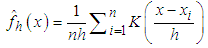(1)

where the smoothing parameter h is called the bandwidth and K is generally chosen to be a unimodal probability density symmetric about zero. That is, K is assumed to be an even regular function with unit variance and zero mean. The Kernel K is called regular if it is a square integrated density.

For a practical implementation of KDE, the choice of the bandwidth h is very important. Small h leads to an estimator with a small bias and large variance, whereas large h leads to a small variance at the expense of increase: the bandwidth has to be optimally chosen (Troudi et al. (2008)).

In this case, K satisfies the following conditions, as may be seen below (Sheather and Jones (1991) and Sheather (2004)),

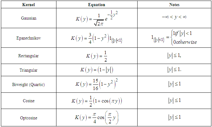
In practice, there are a lot of popular choices of kernel function K such as: Gaussian, Epanechnikov, Rectangular, Triangular, Biweight, Cosine, Optcosine and others, the focus of attention was on this kernels (Silverman (1986)).

The most commonly kernels used have been considered as in Table (1).

Table (1). Kernels under considerations for the kernel density estimation of f (Wolodzko, 2017)

In addition, the bandwidth controls the smoothness of the density estimate and highly influences its appearance. Selecting a suitable h is a pivotal step in estimating f(x).

Supposing that the underlying density is sufficiently smooth and that the kernel has finite fourth moment, by using Taylor series it can be clearly demonstrated that (Sheather (2004)),

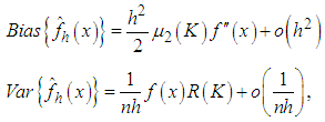where

Adding the leading variance and squared bias terms produces the asymptotic mean squared error (AMSE) as,

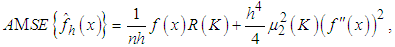An extensively used choice of an overall measure of the discrepancy between and f is the mean integrated squared error (MISE), which is defined by,

Under an integrability assumption on f , integrating the expression for AMSE gives the expression for the asymptotic mean integrated squared error (AMISE), that is,

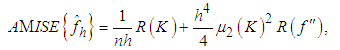(2)

where

In this way, the value of the bandwidth that minimizes the AMISE is obtained by the following

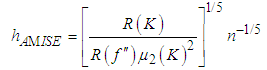supposing that f is sufficiently smooth, we can use integration by parts to demonstrate that,

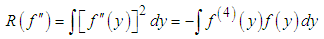Thus, the functional is a measure of the underlying roughness or curvature. In particular, It is clear that the larger the value of is, the larger is the value of AMISE (i.e., the more difficult it is to estimate f ) and the smaller is the value of h_AMISE (i.e., the smaller the bandwidth needed to capture the curvature in f).

Following, we will briefly review some famous methods for choosing a global value of the bandwidth h,

2.1. Rules of Thumb

The computationally simplest method for choosing a global bandwidth h is based on replacing , the unknown part of h_AMISE, by its value for a parametric family expressed as a multiple of a scale parameter, which is then estimated from the data. The method seems to date back to Deheuvels, (1977) and Scott, (1979), who each introduced it for histograms. The method was popularized for kernel density estimates by Silverman, 1986, who used the normal distribution as the parametric family.

Let σ and Q denote the standard deviation and interquartile range of X, respectively. Take the kernel K to be the usual Gaussian kernel. Assuming that the underlying distribution is normal, Silverman, 1986 showed that (2) reduces to,

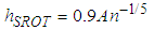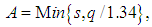where and are sample standard deviation and sample interquartile range respectively. This rule is commonly used in practice and it is often referred to as Silverman’s rule of thumb.

2.2. Cross-Validation Methods

A measure of the closeness of and f for a given sample is the integrated squared error (ISE), which is defined by Bowman, 1984

It is clear that, the last term on the right-hand side of the previous expression does not involve h. Bowman, 1984 presented choosing the bandwidth as the value of h that minimizes the estimate of the two other terms in the last expression, namely,

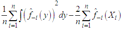where denotes the kernel estimator constructed from the data without the observation x_i. However, the method is commonly referred to as least squares cross-validation, since it is based on the so-called leave-one-out density estimator

Scott and Terrell, 1987 introduced a method called biased cross-validation (BCV), which is based on choosing the bandwidth that minimizes an estimate of AMISE rather than an estimate of ISE. The BCV objective function is just the estimate of AMISE obtained by replacing in (2) by

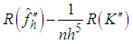where is the second derivative of the kernel density estimate (1) and the subscript h denotes the fact that the bandwidth used for this estimate is the same one used to estimate the density f itself. The BCV objective function is thus defined by Scott and Terrell, 1987

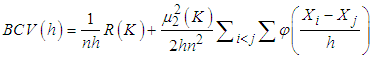Where 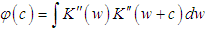. We denote the bandwidth that minimizes by It can be seen that, the above methods are well-known first generation methods for bandwidth selection. These methods were mostly introduced before 1990.

Following some of second generation methods, which are introduced after 1990.

2.3. Smoothed Bootstrap

One approach to this method is to consider the bandwidth that is a minimizer of a smoothed bootstrap approximation to the MISE. Early versions of this were presented by Faraway and Jhun, 1990. An interesting feature of this approach is that unlike most bootstrap applications, the MISE in the "bootstrap world can be calculated exactly, instead of requiring the usual simulation step, which makes it as computationally fast as other methods discussed here. Furthermore, the basic idea behind bootstrap smoothing is very simple, we estimate by a bootstrap version of the form,

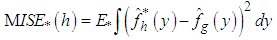where denotes the expectation with respect to the bootstrap sample , g is some pilot bandwidth, is a density estimate which depends on the original sample and is an estimate, based on . Then, we choose the value h minimizing . The basic differences among the various versions of this bootstrap methodology lie on the choice of the auxiliary window g and on the procedure (smoothed or not) for generating the resampled data . Here we introduced a smoothed bootstrap procedure (Smoothed bootstrap with pilot bandwidth) which is considered by Faraway and Jhun, 1990 (the bootstrap sample is taken from ) where g is chosen by least-squares cross-validation from . These authors do not use an exact expression for They approximate by resampling; that is, B bootstrap samples are drawn from , and is approximated by,

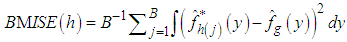Where denotes the value of the estimator for the j-th bootstrap sample. The resulting bandwidth h, is defined as the value of h which minimizes .

2.4. Plug-in Methods

The slow rate of convergence of LSCV and BCV encouraged much research on faster converging methods. A popular approach, commonly called plug-in methods, is to replace the unknown quantity in the expression for given by (2) with an estimate. We next describe the “solve the-equation” plug-in approach developed by Sheather and Jones, 1991, since this method is widely recommended (e.g., Bowman and Azzalini, 1997). The Sheather and Jones, 1991 approach is based on writing g, the pilot bandwidth for the estimate as a function of h, namely,

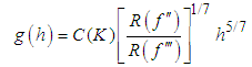The Sheather–Jones plug-in bandwidth h_SJ is the solution to the above equation.

3. Bivariate Kernel Density Estimation

In the bivariate case the data points are considered by two vectors and where is a sample from a bivariate distribution f. In analogy with the univariate case, the bivariate kernel density estimate is given by the following equation (Bilock et al. (2016))

(3)

Here the bandwidth is the positive definite matrix,

and the kernel function K is a symmetric and non negative function fulfilling such that .

As in the univariate case the bivariate kernels used in this work have been the Gaussian kernel, and the Epanechnikov kernel , and other bivariate kernels. To evaluate the closeness of a kernel density estimator to the target density an error criteria must be used. A common error estimate for kernel density estimation is the Mean Integrated Square Error (MISE) which is defined by (Bilock et al. (2016)):

In this case, since the Mean Integrated Square Error depends on the true density f it can only be computed for data sets drawn from known distributions f. The Mean Integrated Square Error can be approximated with the Integrated Mean Square Error IMSE. The expression for the Integrated Mean Square Error IMSE is extracted by moving the expectation value in above equation inside the integral. The IMSE can be computed numerically using Monte Carlo integration, for example. In the bivariate case the plug in method aims to minimize the bivariate AMISE, that is:

where vech represents the following operation

The matrix is given as

where

and

is the partial derivatives of x with respect to and .

Thus, As in the univariate case has to be estimated. A commonly used estimate is

where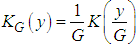

and G is the pilot bandwidth matrix. In Doung and Hazelton (2003), it is proposed that this matrix should be on the form . Choosing g can be done in a similar way as in the univariate case. For each entry in , is chosen such that it minimises the Asymptotic Mean Square Error approximation

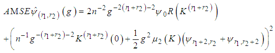This method may produce matrices that are not positive definite. In that case a minimum to the objective function does not exist. To solve this issue, many researchers such as Doung and Hazelton propose a new approach as opposed to finding one optimal g for each entry in . Instead, that minimizes the sum

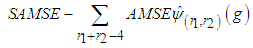should be calculated and used as a common for all entries in . A closed form expression for is given in Doung and Hazelton (2003). In analogy with the univariate case, the estimates of g depends on and therefore an easy estimate of has to be made at some stage (Bilock et al. (2016)).

4. The Proposed Algorithm

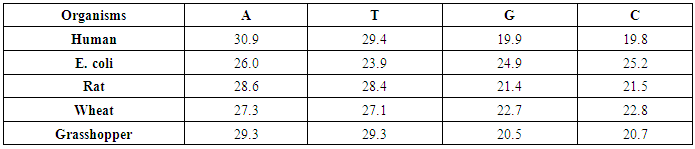
The following algorithm steps is performed to achieve our aims

1. Generate the DNA sequence for five organisms, Human, E. coli, Rat, Wheat and Grasshopper with corresponding information in table (2).

Table (2). Relative proportions (%) of Bases in DNA

2. The sequence size is n=500 and run size is k=205.

3. Transform DNA sequence to numerical values by setting one to the base that appears and zero to the other bases.

4. Transform the sequence of numerical values to the corresponding FFT values.

5. Calculate the eigenvalues of variance covariance matrix for each run results, and then we get 205 fourth order vectors of eigenvalues for each organism. Each vector contains the four eigenvalues, rank from the largest one to the smallest.

5. An Empirical Study and Results Discussion

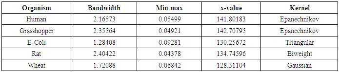
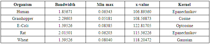
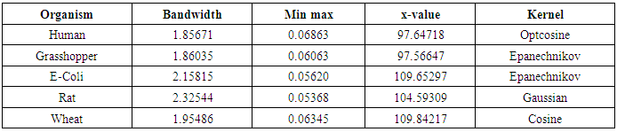
5.1. Univariate Density Estimation

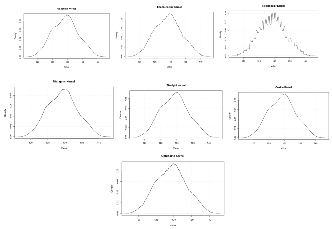
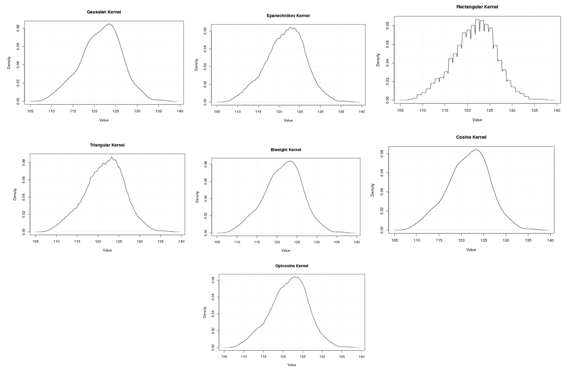
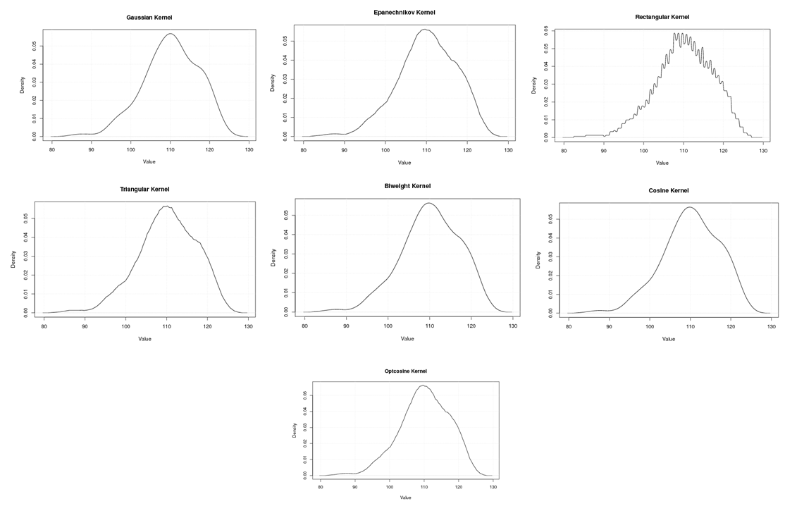
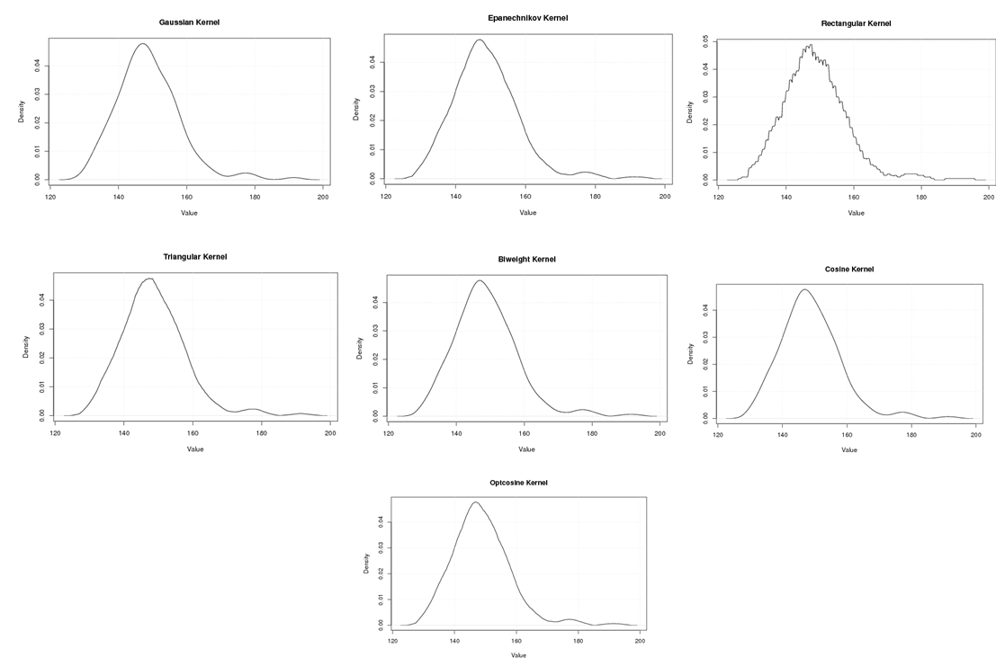
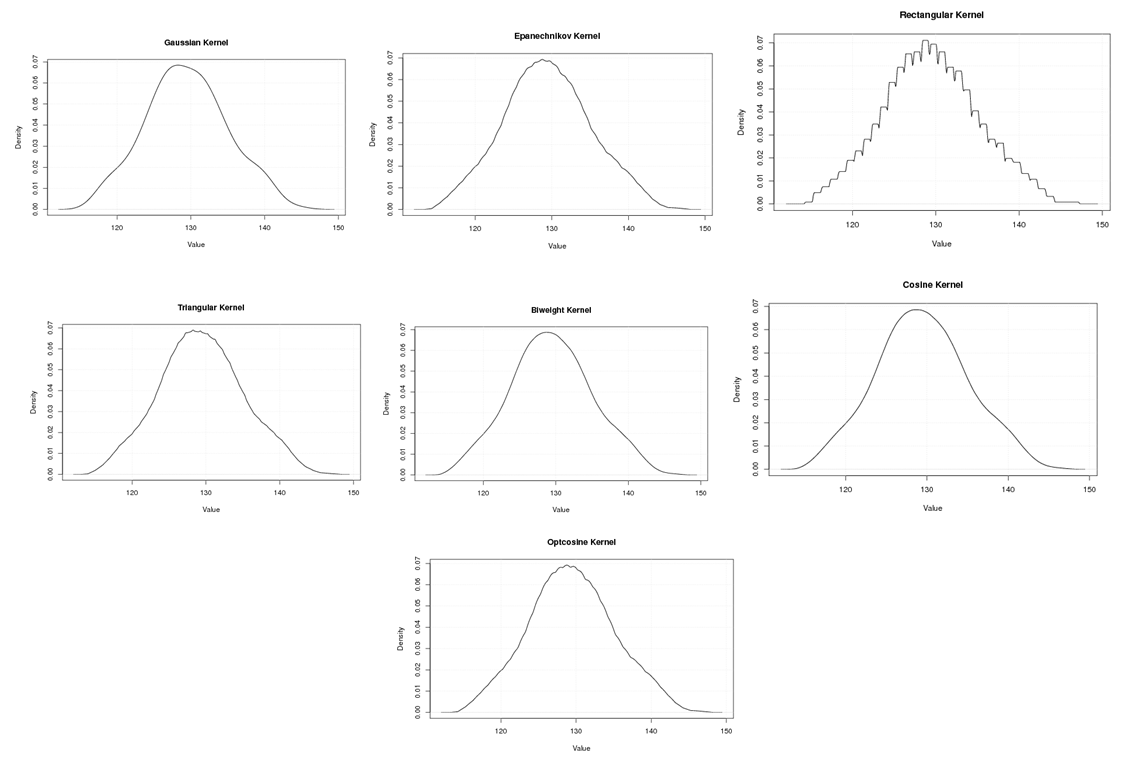
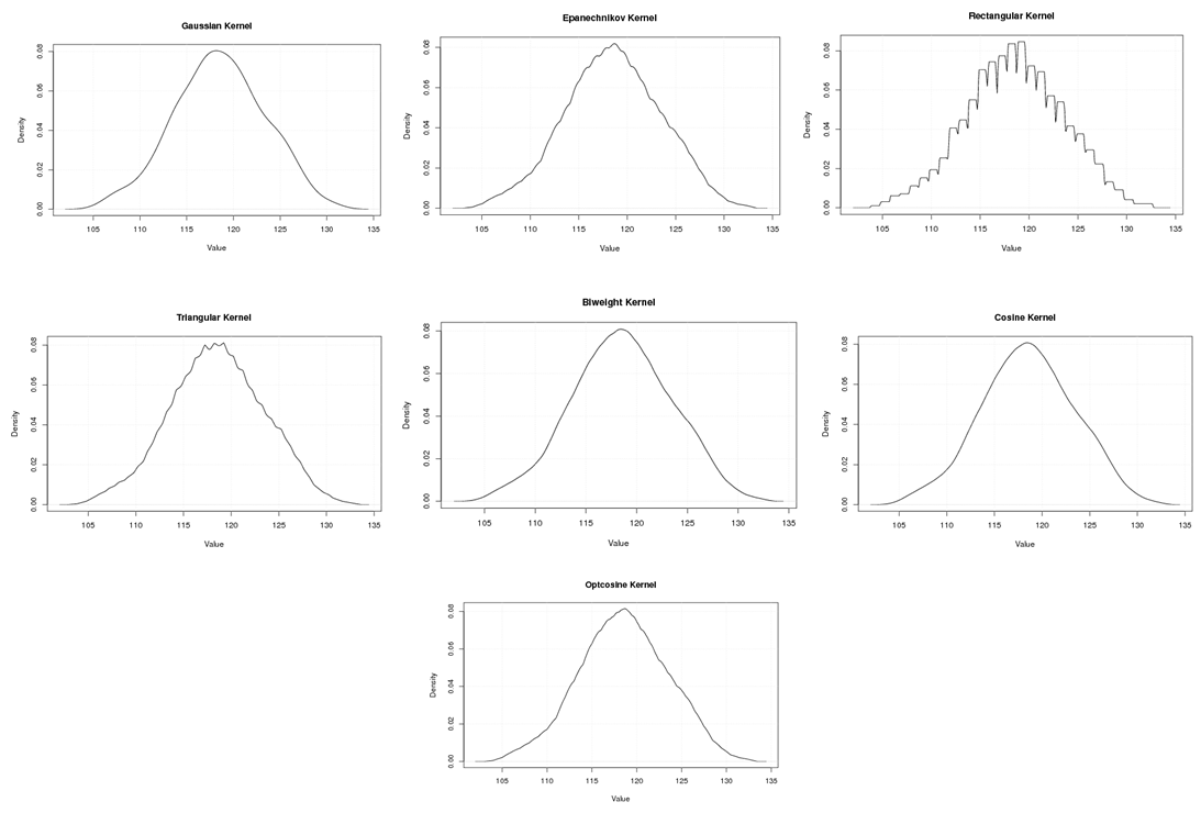
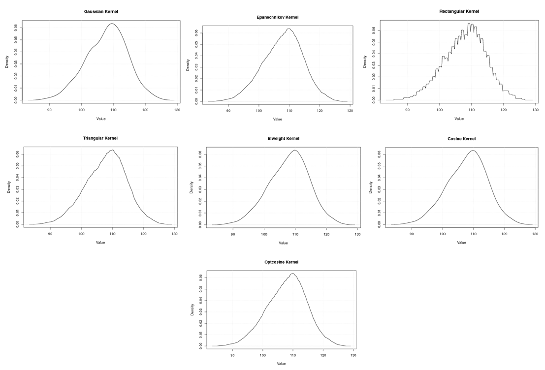
The nonparametric method (kernel density estimation) has been applied of the first, second, third and fourth eigenvalues of variance - covariance matrix of Fast Fourier Transform (FFT) for numerical values representation of DNA sequences of five organisms, Human, E. coli, Rat, Wheat and Grasshopper. It should be noted that it is the first time that the variance covariance matrix eigenvalues of Fast Fourier Transform (FFT) for numerical values representation of DNA sequences, is used in an analysis like this and related analyzes.

We compute an empirical values for the kernel density estimation for data series according to the following Kernels: Gaussian, Epanechnikov, Rectangular, Triangular, Biweight, Cosine, and Optcosine. The results of simulaion experiment are recorded in variety of tables as may be seen below that is, the results is displayed in a series of images. This section summarizes the results of this work by table (8) in appendix (1) and represented in Figures (12 – 31) in appendix (2).

Tables (3 - 6) shows an optimal kernel estimation among kernels under considerations, which are commonly used for these purposes worldwide.

Table (3). Min Max density (at corresponding x-value) and bandwidth for a kernel among kernels under consideration of the first eigenvalue for each organism

Table (4). Min Max density (at corresponding x-value) and bandwidth for a kernel among kernels under consideration of the second eigenvalue for each organism

Table (5). Min Max density (at corresponding x-value) and bandwidth for a kernel among kernels under consideration of the third eigenvalue for each organism

Table (6). Min Max density (at corresponding x-value) and bandwidth for a kernel among kernels under consideration of the fourth eigenvalue for each organism

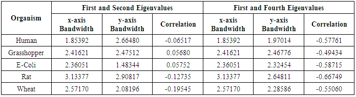
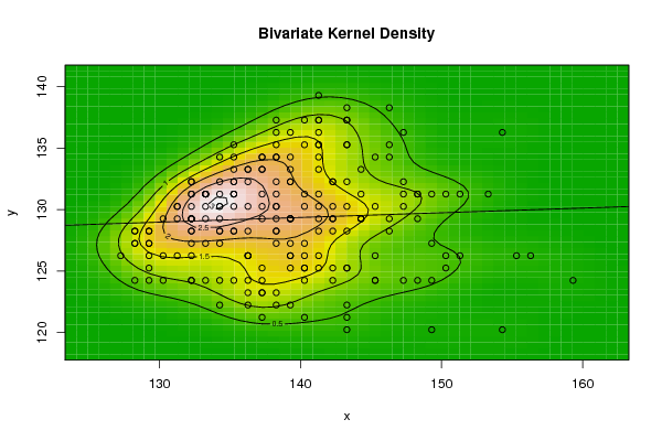
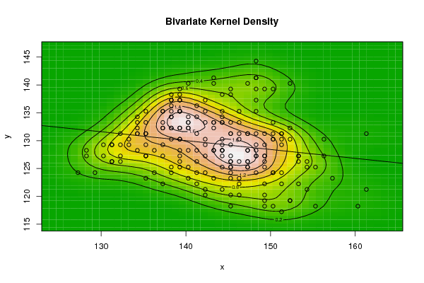
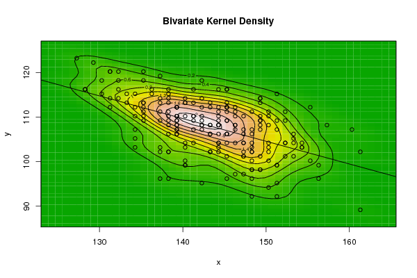
5.2. Bivariate Density Estimation

The bivariate kernel density estimation has been applied of the first and second eigenvalues from a side and the first and fourth eigenvalues from another side. These eigenvalues of variance covariance matrix of Fast Fourier Transform for numerical values representation of DNA sequences of five organisms, Human, E. coli, Rat, Wheat and Grasshopper.

Table (7) contain the results referred to below.

Table (7). Empirical values for the Bandwidth and Correlation used in KDE of each of five organisms

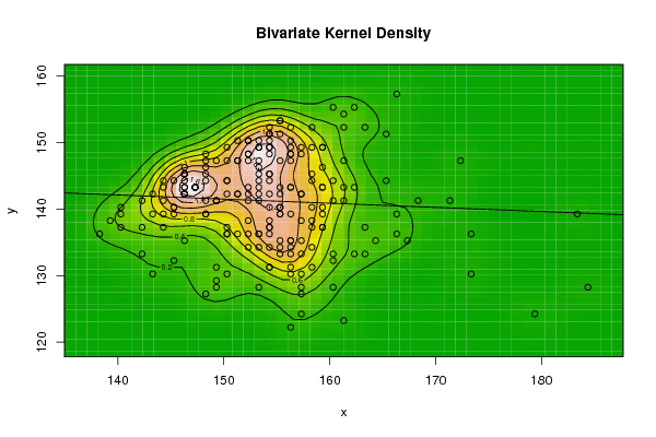Figure 2. Plot of bivariate kernel density for Human according to first and second eigenvalues

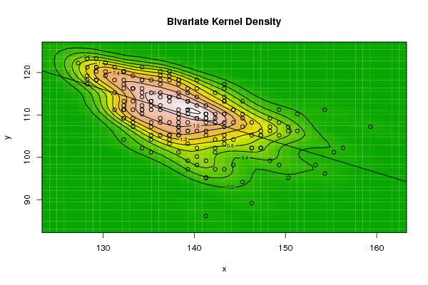
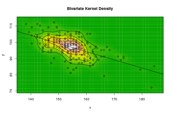Figure 3. Plot of bivariate kernel density for Human according to first and fourth eigenvalues

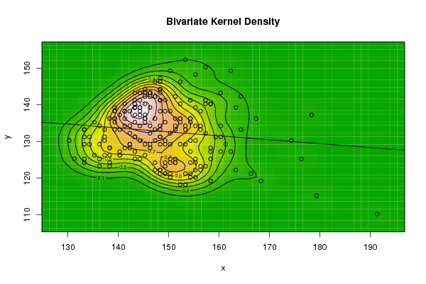
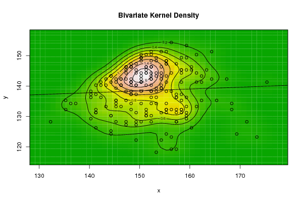Figure 4. Plot of bivariate kernel density for Grasshopper according to first and second eigenvalues

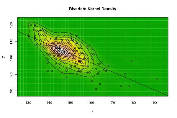
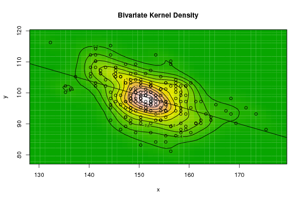Figure 5. Plot of bivariate kernel density for Grasshopper according to first and fourth eigenvalues

Figure 6. Plot of bivariate kernel density for E-Coli according to first and second eigenvalues

Figure 7. Plot of bivariate kernel density for E-Coli according to first and fourth eigenvalues

Figure 8. Plot of bivariate kernel density for Rat according to first and second eigenvalues

Figure 9. Plot of bivariate kernel density for Rat according to first and fourth eigenvalues

Figure 10. Plot of bivariate kernel density for Wheat according to first and second eigenvalues

Figure 11. Plot of bivariate kernel density for Wheat according to first and fourth eigenvalues

The results in table (7) and plots will be crucial to determine DNA afiliation.

6. Summary

One of important properties of FFT, which is return the variations to their original sources help us tremendously to understand, discriminant and deal with DNA sequences.

Probability behavior of DNA data, represented by the density estimation, is very important. The references stated here, highlights some aspects of that importance.

Univariate density estimation is fitted for first, second, third and fourth eigenvalues of variance covariance matrix of Fast Fourier Transform for numerical values representation of DNA sequences of five organisms, Human, E. coli, Rat, Wheat and Grasshopper.

Bivariate density estimation is fitted for first and second eigenvalues from a side and first and fourth eigenvalues from another side. We treat here with first and second eigenvalues from a side and first and fourth eigenvalues from another side because we think that the relations between them are more interactive than others. These eigenvalues of variance covariance matrix of Fast Fourier Transform for numerical values representation of DNA sequences of five organisms, Human, E. coli, Rat, Wheat and Grasshopper.

The methods used here are aimed to discriminant among different organisms using another point of view. This point of view is based on eigenvalues of variance covariance matrix of FFT for numerical values representation of DNA sequences. It should be noted that, it is the first time this point of view is used to achieve aims like ours.

Empirical studies are conducted to show the value of our point of view and the applications based on. So we recommended that,

(1) Other empirical studies should be done for other organisms and statistical methods by using the point of view adopted here.

(2) Aspects stated here must be used in an applied manner for DNA sequences discrimination.

Appendix (1)

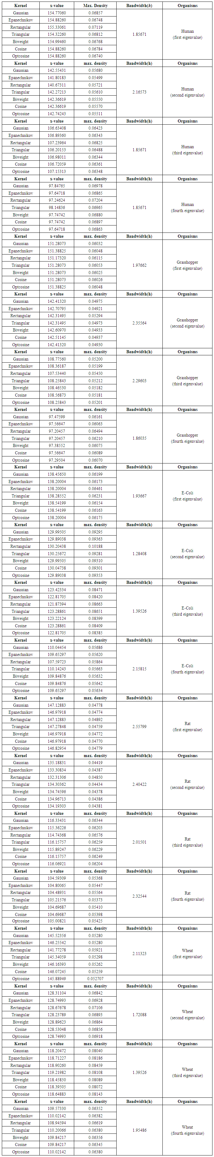Table (A.1). Empirical values of maximum density and bandwidth for the (first, second, third and fourth) eigenvalues of each of five organisms

Appendix (2)

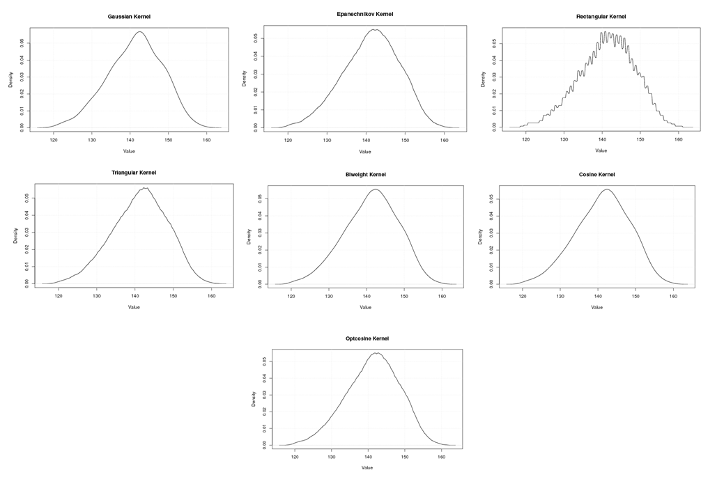
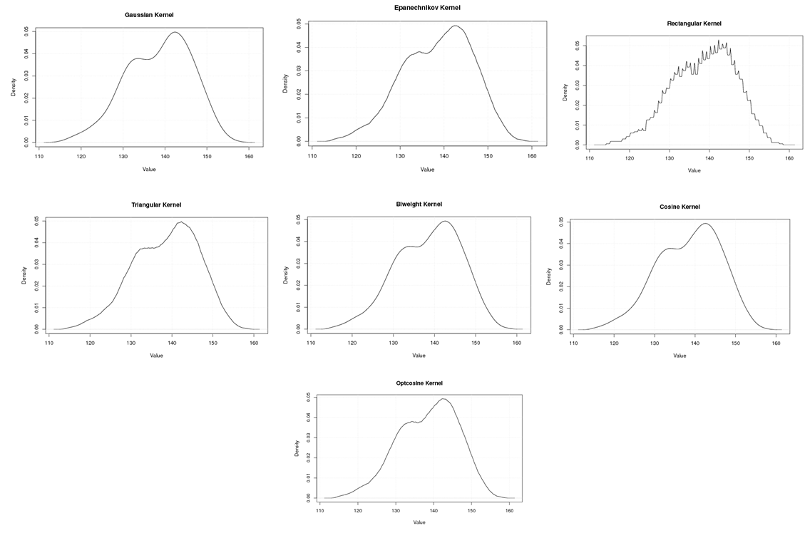
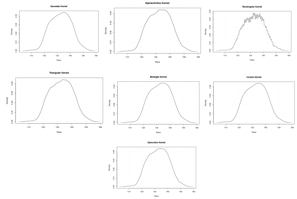
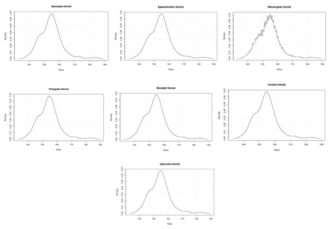Figure A.1. Kernel density estimation plots for the first eigenvalue of Human according to Gaussian, Epanechnikov, Rectangular, Triangular, Biweight, Cosine, and Optcosine kernels

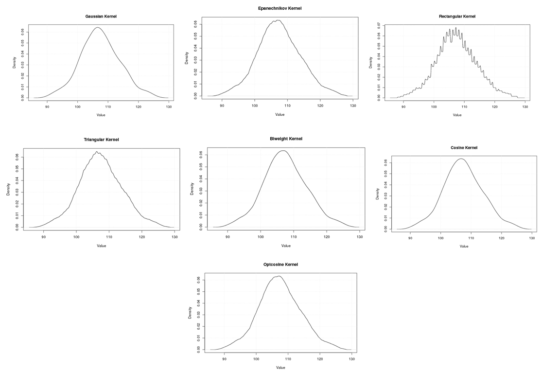
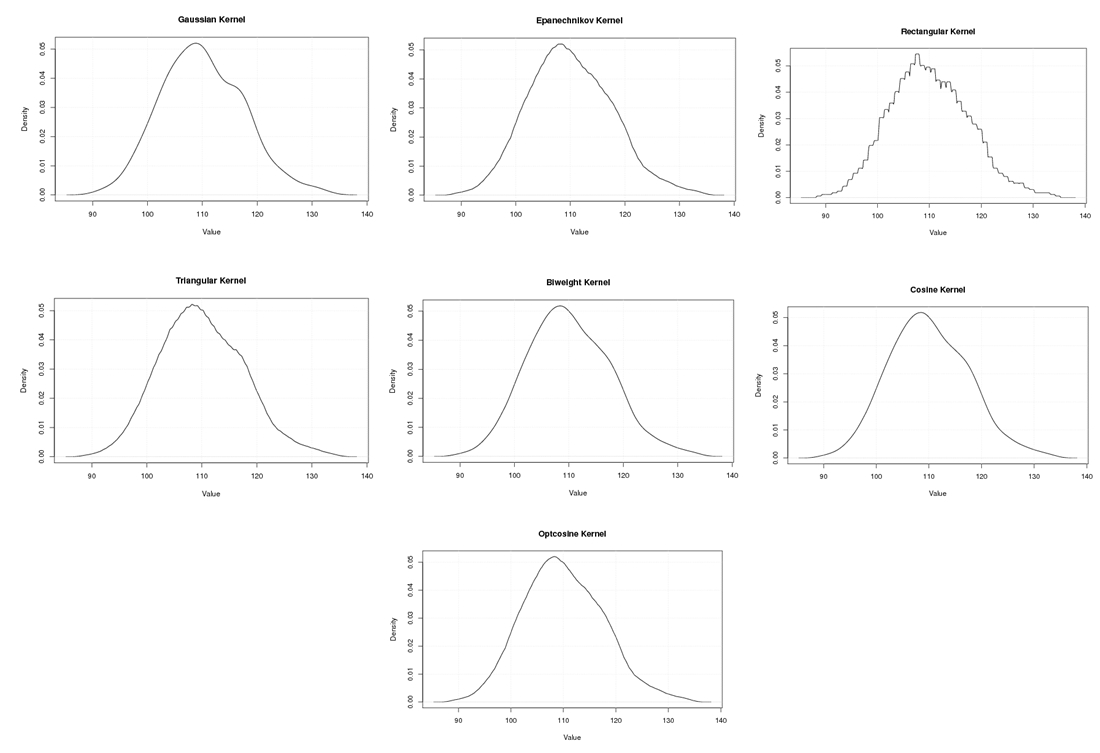
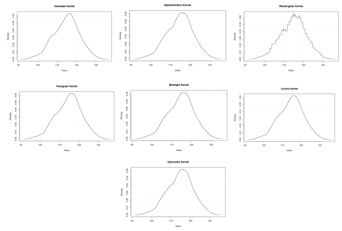
Figure A.2. Kernel density estimation plots for the second eigenvalue of Human according to Gaussian, Epanechnikov, Rectangular, Triangular, Biweight, Cosine, and Optcosine kernels

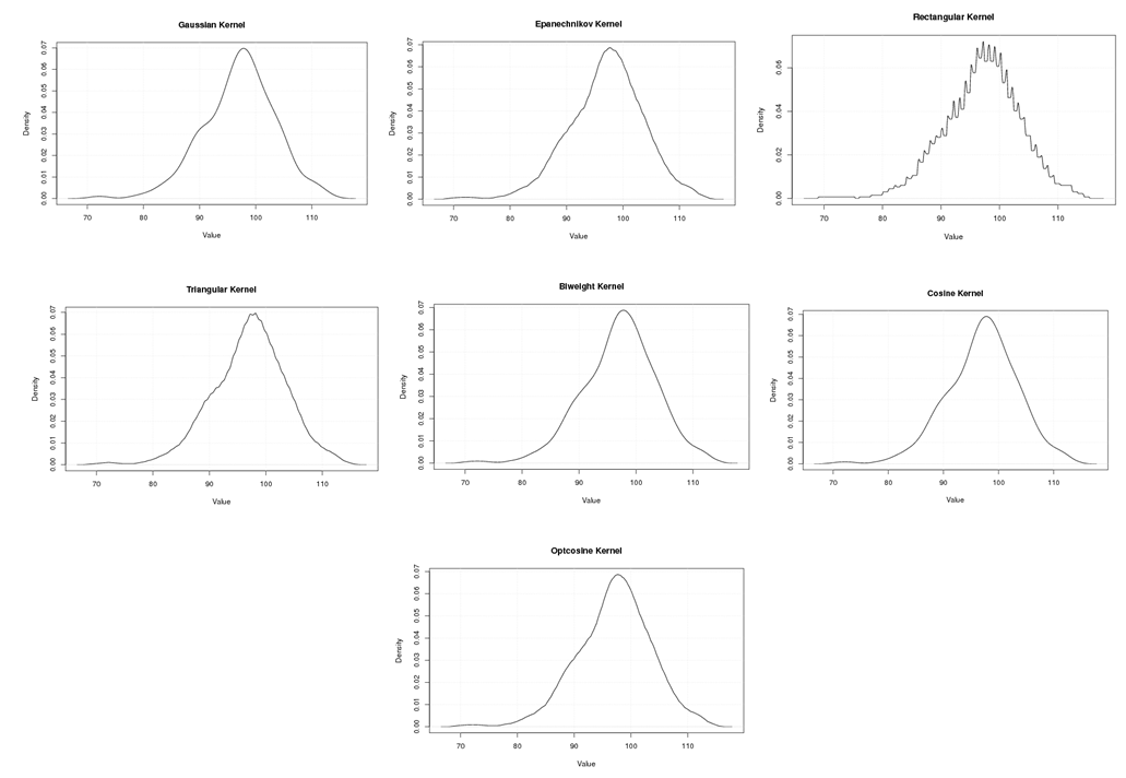
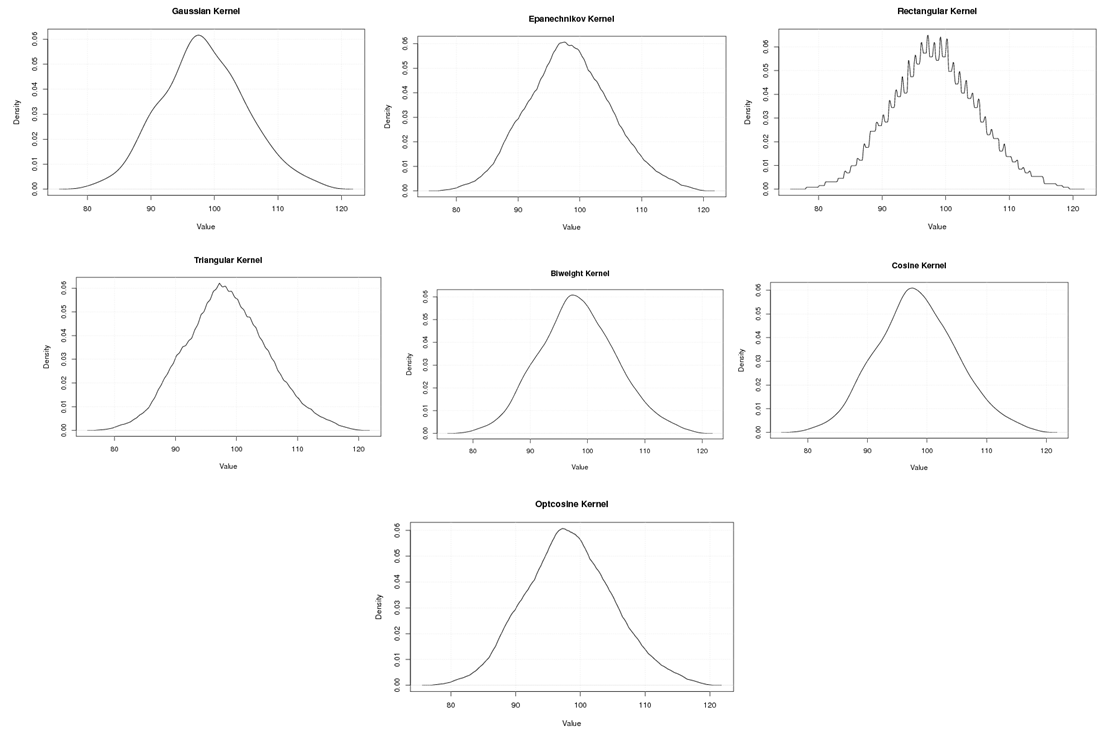
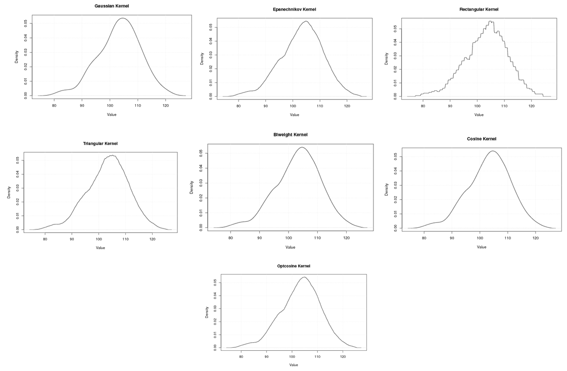
Figure A.3. Kernel density estimation plots for the third eigenvalue of Human according to Gaussian, Epanechnikov, Rectangular, Triangular, Biweight, Cosine, and Optcosine kernels

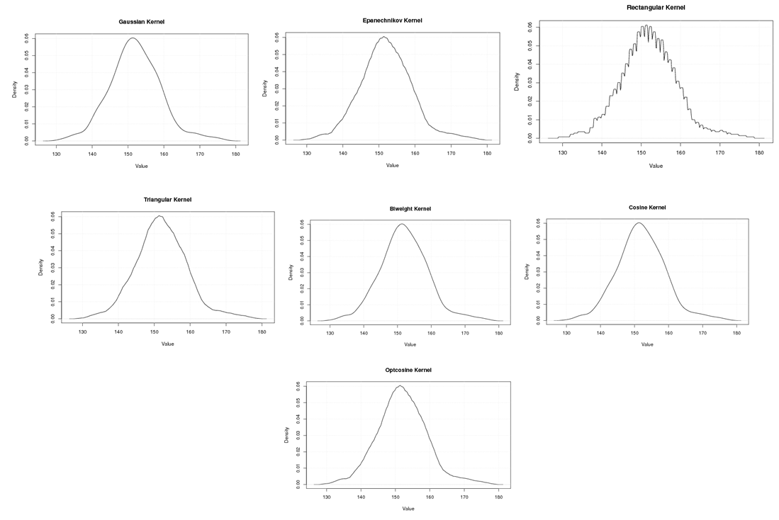
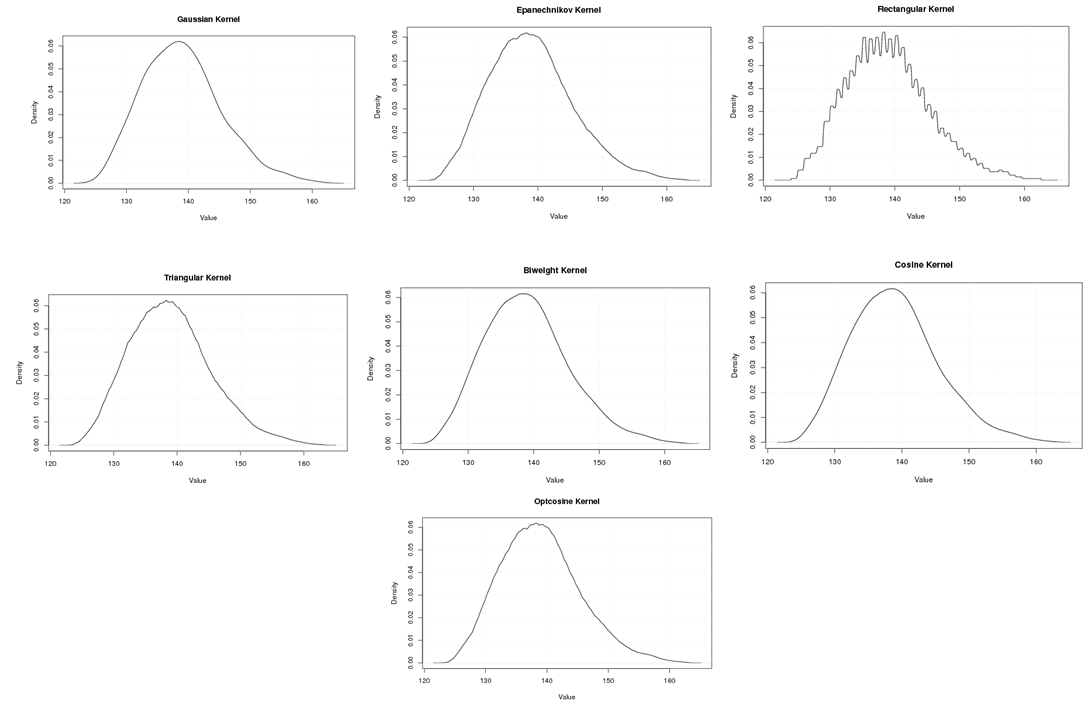
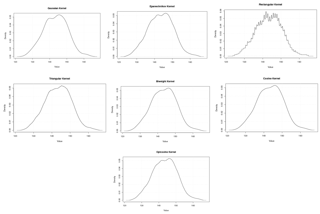
Figure A.4. Kernel density estimation plots for the fourth eigenvalue of Human according to Gaussian, Epanechnikov, Rectangular, Triangular, Biweight, Cosine, and Optcosine kernels

Figure A.5. Kernel density estimation plots for the first eigenvalue of Grasshopper according to Gaussian, Epanechnikov, Rectangular, Triangular, Biweight, Cosine, and Optcosine kernels

Figure A.6. Kernel density estimation plots for the second eigenvalue of Grasshopper according to Gaussian, Epanechnikov, Rectangular, Triangular, Biweight, Cosine, and Optcosine kernels

Figure A.7. Kernel density estimation plots for the third eigenvalue of Grasshopper according to Gaussian, Epanechnikov, Rectangular, Triangular, Biweight, Cosine, and Optcosine kernels

Figure A.8. Kernel density estimation plots for the fourth eigenvalue of Grasshopper according to Gaussian, Epanechnikov, Rectangular, Triangular, Biweight, Cosine, and Optcosine kernels

Figure A.9. Kernel density estimation plots for the first eigenvalue of E-Coli according to Gaussian, Epanechnikov, Rectangular, Triangular, Biweight, Cosine, and Optcosine kernels

Figure A.10. Kernel density estimation plots for the second eigenvalue of E-Coli according to Gaussian, Epanechnikov, Rectangular, Triangular, Biweight, Cosine, and Optcosine kernels

Figure A.11. Kernel density estimation plots for the third eigenvalue of E-Coli according to Gaussian, Epanechnikov, Rectangular, Triangular, Biweight, Cosine, and Optcosine kernels

Figure A.12. Kernel density estimation plots for the fourth eigenvalue of E-Coli according to Gaussian, Epanechnikov, Rectangular, Triangular, Biweight, Cosine, and Optcosine kernels

Figure A.13. Kernel density estimation plots for the first eigenvalue of Rat according to Gaussian, Epanechnikov, Rectangular, Triangular, Biweight, Cosine, and Optcosine kernels

Figure A.14. Kernel density estimation plots for the second eigenvalue of Rat according to Gaussian, Epanechnikov, Rectangular, Triangular, Biweight, Cosine, and Optcosine kernels

Figure A.15. Kernel density estimation plots for the third eigenvalue of Rat according to Gaussian, Epanechnikov, Rectangular, Triangular, Biweight, Cosine, and Optcosine kernels

Figure A.16. Kernel density estimation plots for the fourth eigenvalue of Rat according to Gaussian, Epanechnikov, Rectangular, Triangular, Biweight, Cosine, and Optcosine kernels

Figure A.17. Kernel density estimation plots for the first eigenvalue of Wheat according to Gaussian, Epanechnikov, Rectangular, Triangular, Biweight, Cosine, and Optcosine kernels

Figure A.18. Kernel density estimation plots for the second eigenvalue of Wheat according to Gaussian, Epanechnikov, Rectangular, Triangular, Biweight, Cosine, and Optcosine kernels

Figure A.19. Kernel density estimation plots for the third eigenvalue of Wheat according to Gaussian, Epanechnikov, Rectangular, Triangular, Biweight, Cosine, and Optcosine kernels

Figure A.20. Kernel density estimation plots for the fourth eigenvalue of Wheat according to Gaussian, Epanechnikov, Rectangular, Triangular, Biweight, Cosine, and Optcosine kernels