Nickson Cheruiyot, Luke Akong’o Orawo, Ali Salim Islam
Department of Mathematics, Egerton University, Egerton, Kenya
Correspondence to: Nickson Cheruiyot, Department of Mathematics, Egerton University, Egerton, Kenya.
| Email: |  |
Copyright © 2019 The Author(s). Published by Scientific & Academic Publishing.
This work is licensed under the Creative Commons Attribution International License (CC BY).
http://creativecommons.org/licenses/by/4.0/

Abstract
Musa – Okumoto (1984) non-homogeneous Poisson Process (NHPP) software reliability model also known as logarithmic NHPP model is one of the widely used reliability model. The model is based on the assumptions that failures are observed during execution time caused by remaining faults in the software; whenever a failure is observed, an instantaneous effort is made to find what caused the failure and the faults are removed prior to future tests and whenever a repair is done it reduces the number of future faults not like other models. The failure intensity function of this model reduces exponentially with time and the expected number of failures has logarithmic function. The predictive analysis of software reliability model is of great importance for modifying, debugging and determining when to terminate software development testing process. This paper presents some results about predictive analyses for the Musa – Okumoto (1984) NHPP model. Four issues in single-sample prediction associated closely with development testing program are addressed. Bayesian approach based on informative prior was adopted to develop explicit solutions to the problems which arise during software development testing process. Developed methodologies were illustrated using real data in form of time between failures.
Keywords:
Bayesian approach, Intensity function, Informative prior, Software reliability model
Cite this paper: Nickson Cheruiyot, Luke Akong’o Orawo, Ali Salim Islam, Predictive Analyses of Logarithmic Non – Homogeneous Poisson Process in Software Reliability Using Bayesian Approach with Informative Priors, American Journal of Mathematics and Statistics, Vol. 9 No. 2, 2019, pp. 57-65. doi: 10.5923/j.ajms.20190902.02.
1. Introduction
Developing a reliable software is a challenging task facing software industry. This therefore calls for a method for checking whether the developed software is reliable or not. To determine when to terminate development process of a software there is need to carry out predictive analyses. Bayesian predictive analyses using various software reliability growth models has attracted a number of researchers. For instant, predictive analyses for the power law process (PLP) was developed, where most problems that relates to development process of software were solved using Bayesian approach [1]. [2] also solved the issues related to software development process by conducting a Bayesian predictive analyses for Goel- Okumoto software reliability growth model. Both models assume that failures are finite and that a software can be free of errors at a given time when all faults have been removed which might not happen at a real situation. Predictive analyses for Musa – Okumoto software reliability growth model has not been developed and the model assume failures to be infinite, that is there is no point in time a software will have zero faults, which is true in real situation. The model assumes that the earlier faults that are removed have great impact than the remaining faults. The Musa – Okumoto software reliability model is one of non-homogeneous Poisson process software model with the intensity function given by; | (1) |
The model is based on the assumptions that failures are observed during execution time caused by remaining faults in the software; whenever a failure is observed, an instantaneous effort is made to find what caused the failure and the faults are removed prior to future tests and whenever a repair is done it reduces the number of future faults not like other models. The model must remain stable during the entire testing period for any particular testing environment and a reasonably accurate prediction of reliability must be provided by the model. These are the two main aspects of a good reliability model [3]. The Musa – Okumoto (1984) model has been used in various testing environment and in many instances, it provides good estimation and prediction of software reliability. Compared to other models when used in testing industrial data set, Musa- Okumoto model is the best performer in terms of fitting and predictive capability to the data [4].Bayesian reliability modeling is one of the best methods in predictive analysis. Development of reliability posterior distribution from which predictive inference is made is the main thing required in Bayesian reliability model. The reliability posterior distribution is usually constructed using prior distribution for the parameters of the software reliability model and the likelihood function based on the observed data. The advantage of using Bayesian approach is that it allows prior information such as engineering judgments and test results to be combined with more recent information from test or field data. This is vital since it helps software developers to arrive at a prediction of reliability based upon a combination of all available information. This information includes; the environment under which the software will work, previous tests on the software and even intuition based upon experience [5]. This paper present single – sample prediction analyses for Musa – Okumoto model using Bayesian approach with informative priors.
2. Bayesian Method
Computer Software is an important complex intellectual product that has become driver of almost everything in the 21st century. During its development testing, developers and statisticians are interested on some prediction problems that are believed to be helpful in modifying the development testing program. In this section we present four issues A, B, C and D in single – sample prediction associated closely to development testing program. The four issues that were addressed are outline as propositions and their proof given in the appendix. Predictive distributions were derived using Bayesian method with informative priors. In this paper, it is assumed that a reliability growth testing is performed on a computer software system and the number of failures in the time interval  , denoted by
  is observed. It is also assumed that
  follows the NHPP with intensity given in equation (14). Let
  be the successive failure times. When testing stops after a pre-determined
  number of failures is observed, the failure data is said to be failure-truncated. We denote the
  failures time by
  where
where  a time-truncated data is when testing is observed for fixed time
  . We denote the corresponding observed data by
  , where
  A prediction interval is an interval estimate for a future observation or a function of some future observations (Jun – Wu et al., 2007). Specifically, a double-sided (bilateral) prediction interval for
  a future failure time with confidence level
  is defined by
  where
where  and
and  are the lower and upper prediction limits respectively such that
 Similarly, a single-sided (unilateral) lower or upper prediction limit for
  with level
  is defined by
  (or
(or  ), which satisfies
 or
or  Both lower and upper prediction limits,
  and
and  respectively, depend only on a single sample (or a single software) and are called single-sample prediction limits. Prediction limits involving two samples (or two software) can be defined similarly and are called two-sample prediction limits.
2.1. Predictive Issues
Here, we consider one software and assume that its cumulative time between failure times obey Musa – Okumoto software reliability growth model with observed data as either  or
or  . Based on
  or
or  , we are interested in the following problems:A: What is the probability that at most k software failure will occur in the future time period
  with
with  ?B: Given that the pre-determined target value
  for the failure rate of the software undergoing development testing is not achieved at time T, what is the probability that the target value
  will be achieved at time
  C: Suppose that the target value
  for the software failure rate is not achieved at time T, how long will it take so that the software failure rate will be attained at
  D: What is the upper prediction limit (UPL) of
 with level
  being a pre-determined value greater than T?
2.2. Posterior and Predictive Distribution
Let  represent
  or
or  . The joint density distribution of
  is therefore [6]:
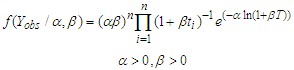 | (2) |
Case 1: When  the shape parameter is known, we adopt the following an informative prior for
  , that is
 , where
  and
and  are known
 | (3) |
The posterior of  is thus obtained as
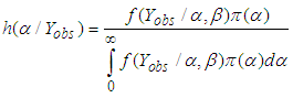 | (4) |
Substituting equation (2) and equation (3) into equation (4) we have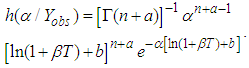 | (5) |
Let  be the random variable being predicted. The predictive density of
  is;
is;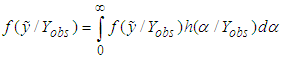 | (6) |
Hence, the Bayesian UPL of  with level
  , denoted as
  , must satisfy
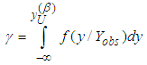 | (7) |
Case 2: Shape parameter  is unknown, we assume the informative priors for
  and
and  as
as  and
and . This implies that
  and
and  . Since
  and
and  are independent the joint prior density
  is given as
 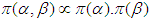 . Implying that
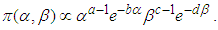 | (8) |
The joint posterior density of  and
and  is thus
 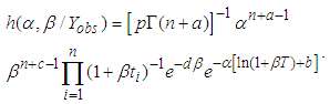 | (9) |
where 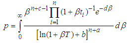 Equation (9) is similar to equation (5), let
  be the random variable predicted. The predictive density of
  is;
is; | (10) |
and the Bayesian UPL denoted by  of
of  with level
  similar to equation (6) is;
 | (11) |
3. Main Results for Prediction Using Informative Priors
In this section we address the four issues stated in section 2.1 using the Bayesian approach. The main results are presented as propositions and their proofs given in the appendix. Below, we use  to represent
  the percentage point of the chi-square distribution with degrees of freedom such that
  , and define the Poisson mass function as
  and gamma density function as
  . The prior is assumed to be equation (3) and (8) in all subsequent propositions. Preposition 1 (Issue A)The probability that at most
  failures will occur in the interval
  with
with  is
is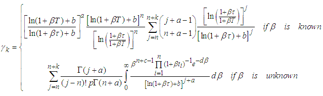 | (12) |
Preposition 2 (Issue B)The probability that the target value  will be achieved at time
  is
is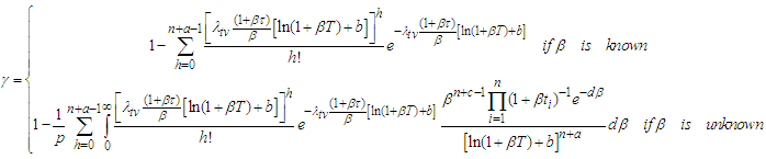 | (13) |
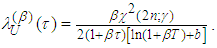
Preposition 3 (Issue C)For a given level  , the time
  required to attain
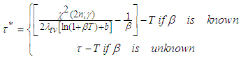 | (14) |
Remark 1: For the second part of equation (14),  is the solution to the equation
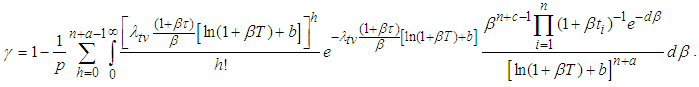 | (15) |
Preposition 4 (Issue D)The Bayesian UPL of  with level
  is
is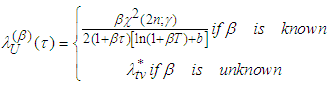 | (16) |
Remark 2: The second part of equation (16) is such that  is the solution to
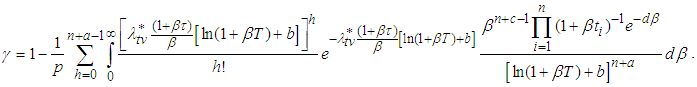 | (17) |
4. Real Example
We have used the time between failures data described in [7] to illustrate the developed methodologies for the single-sample Bayesian predictive analysis. We conducted the goodness of fit test using Laplace statistics as presented in [8] and found that the data obey the Musa – Okumoto process. From the given data the maximum likelihood estimates for the parameters  and
and  of Musa – Okumoto growth model were obtained numerically by Newton Raphson method as
  and
and  respectively. In this paper we have used gamma priors for both parameters. The values of the parameters of informative priors
  and
and  are chosen arbitrarily as
  and
and  .(A) Suppose we are interested in the probability
  that at most
  will occur in a future time period
  . Considering the case when
  is known (i.e,
  ), using the first formula in equation (12) we have
 Figure 1 shows the graph of probabilities that at most
  failures will occur in the time interval for
  known for both informative and non-informative priors. From the graph it can be seen that the probabilities for informative prior is high as compared to that of non-informative. This is more seen at issue C, where there high reduction of time required to achieve a predetermined target value in informative prior.(B) Suppose the target value is given by
  . At the time
  , the MLE of the achieved failure rate for this software is
  which is greater than
  thus it cannot be achieved at time
  and development testing will continue. Suppose we want to find the probability that the target value
  will be achieved at the time
  . (i) When
  is known (say,
  ), from the first formula in equation (13), we obtain
  . In this case also as that of non-informative prior, the target value is unlikely to be achieved. (ii) When
  is unknown, from the second formula in equation (13), we obtain
 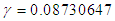 where the Monte Carlo sample size
  .
. 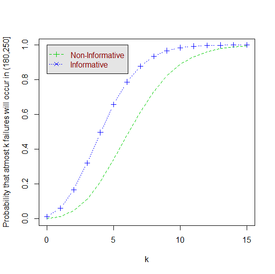 | Figure 1. The graph of the probabilities  that at most that at most  failures will occur in the time interval (180, 250] for the cases of failures will occur in the time interval (180, 250] for the cases of  known for informative and non-informative prior known for informative and non-informative prior |
(C) Since the target value  is not achieved at time
  . It is interesting now to know how long it will take in order to achieve the desired target value. (i) When
  is known (say,
 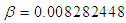 ), using the first formula in equation (14) and letting
  , we obtain
 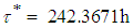 . Thus, it will take another
  hours in order to achieve the target value which is a significant reduction from the value obtained for the case of non-informative prior. (ii) When
  is unknown, from the second formula in equation (14) we have
  . It will take another hours for the desired target value to be achieved when
  is unknown. . (D) Given
  , when
  is known (i.e,
  ), from first formula in equation (16) the Bayesian UPL of
  with level
  is given by
  .
.
5. Conclusions
Reliable software has been the main goal of any software developer. This is because non- reliable software means that the customers will be dissatisfied with the product thus loss of market shares and significant cost to the supplier. For critical applications such as banking or health monitoring, non-reliability can lead to great damage not only to the consumer but also to the developer. Due to the above reasons, there is need to develop reliable software. There are many software reliability growth models that have been used in analyzing software reliability data. Musa- Okumoto is one of the software reliability models which best performed in fitting industrial failure data set. In this paper, explicit solution to predictive issues that may arise during development process were derived using Bayesian approach. These solutions are helpful to software developers in many instances such as resource allocation, when to terminate the testing process, modification needed in the software before termination. The study used informative to derived explicit solutions for predictive issues that may arise during software development process. In all the cases when the shape parameter was known, solutions to posterior and predictive distributions had closed forms while when it is unknown, solutions had no closed forms and the study used Markov Chain Monte Carlo (MCMC). Bayesian approach was used as it is advantageous over classical approach. Bayesian approach is available for small sample sizes and allows the input of prior information about reliability growth process and provides full posterior and predictive distributions [1].
Appendix: Proof of preposition 1 – 4
We first state the following identity without proof: That is | (A.1) |
where  is any positive integer,
  and
and  are two real numbers such that
  is an increasing and differentiable function and
  Proof of preposition 1The probability that at most
  failures will occur in the interval
  is
is  , when
  is known, we have
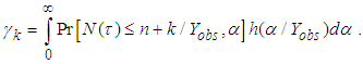 | (A.2) |
where  is given by equation (5) and
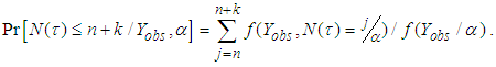 | (A.3) |
From equation (2) 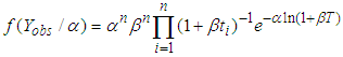 and
and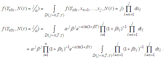 | (A.4) |
Solving the integral part in equation (A.4), we proceed as follows: . Substituting the limits
  and
and  we have
  which reduces to
  . Therefore the integral part of equation (A.4) becomes
 | (A.5) |
Substituting equation (A.5) to equation (A.4) we have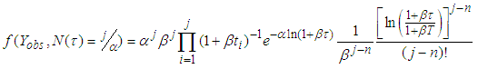 From equation (A.3), we obtain
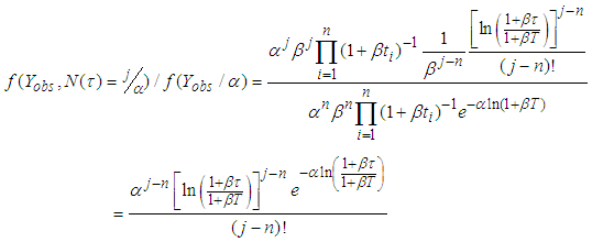 Thus equation (A.3) becomes
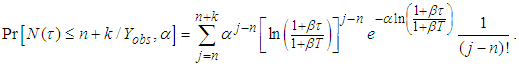 | (A.6) |
and equation (A.2)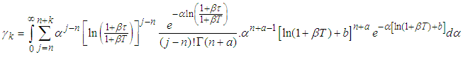 | (A.7) |
The integral part of equation (A.7) integrates to 1 since it is a gamma distribution with parameters  and
and . On re-arranging equation (A.7), it becomes
 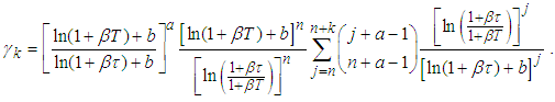 | (A.8) |
This implies the first formula of equation (12).When  is unknown, from equation (9) and equation (A.6) we have
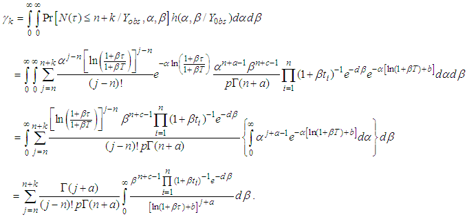 | (A.9) |
Equation (A.9) implies the second formula of equation (12). Proof of Preposition 2Let  denote the posterior of
 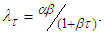 Hence, the probability that the target value
  will be achieved at time
  is given by
 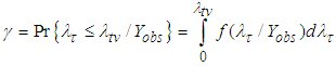 . When
  is known, making transformation
  , we have
  and
and  . Consequently, the posterior density of
  is
is | (A.10) |
Equation (A.10) follows a gamma distribution with parameters  and
and  . From the relationship of gamma and Poisson distribution
  .Thus, we have
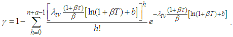 | (A.11) |
Equation (A.11) implies the first formula of equation (13).When  is unknown, making transformation on
  and
and  , we obtain
  and
and  . Note that the Jacobian is
  . From equation (9), the joint posterior density of
  is
is | (A.12) |
We obtain, | (A.13) |
Equation (A.13) implies the second formula of equation (13).Proof of Preposition 3For given level  , the time required to attain the target value
  is
is  , where
  satisfies
 . When
  is known, from equation (A.10), it can easily been seen that
 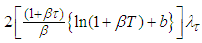 follows a chi-square distribution with
  degrees of freedom. Thus we have
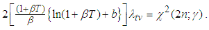 | (A.14) |
Hence  is given as
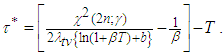 | (A.15) |
When  is unknown, the time required to attain the target value
  with level
  is
is  . Where
  is the solution to
 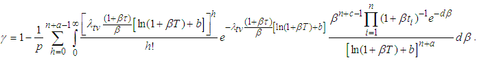 | (A.16) |
Proof of Preposition 4For a pre-determined  , the Bayesian UPL for
  with level
  is
is  satisfying
  . From
  and equation (A.14) we have
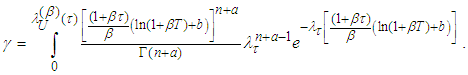 | (A.16) |
 | (A.17) |
Equation (A.17) implies the first formula of equation (16) and the second part follows similarly.
References
| [1] | Jun-Wu, Y., Guo-Liang, T. and Man-Lai, T., (2007). Predictive analyses for non-homogeneous Poisson processes with power law using Bayesian approach. Computational Statistics & Data Analysis, 51: 4254-4268. |
| [2] | Akuno, A.O., Orawo, L.A. and Islam, A.S. (2014) One-Sample Bayesian Predictive Analyses for an Exponential Non-Homogeneous Poisson Process in Software Reliability. Open Journal of Statistics, 4, 402-411. |
| [3] | Ullah, N., Morisio, M. and Vetro, A. (2013). A Comparative Analysis of Software Reliability Growth Models using defects data of Closed and Open Source Software. In: 35TH Annual IEEE Software Engineering Workshop, Heraclion, Crete, Greece, 12-13 October 2012. pp. 187-192. |
| [4] | Kapur, P. K., Pham, H., Gupta, A. and Jha, P. C., (2011). Software Reliability Assessment with OR Applications. Springer Series in Reliability Engineering, Springer-Verlag London Limited 2011. 58. |
| [5] | Allan, T. M., (2012). Bayesian Statistics applied to Reliability Analysis and Prediction. Raython Missile Systems, Tucson, AZ. |
| [6] | Crowder, M. J., Kimber, A., Sweeting, T., & Smith, R. (1994). Statistical analysis of reliability data (Vol. 27). CRC Press. |
| [7] | Xie, M., Goh, T. N., & Ranjan, P. (2002). Some effective control chart procedures for reliability monitoring. Reliability Engineering & System Safety, 77(2), 143-150. |
| [8] | Zhao, J., and Wang, J. (2005). A new goodness-of-fit test based on the Laplace statistic for a large class of NHPP models. Communications in Statistics—Simulation and Computation®, 34(3), 725-736. |

 Abstract
 Reference
 Full-Text PDF
 Full-text HTML