E. O. Eze, U. E. Obasi, S. I. Ezeh
Department of Mathematics, Michael Okpara University of Agriculture Umudike, Umuahia, Abia State, Nigeria
Correspondence to: E. O. Eze, Department of Mathematics, Michael Okpara University of Agriculture Umudike, Umuahia, Abia State, Nigeria.
| Email: |  |
Copyright © 2019 The Author(s). Published by Scientific & Academic Publishing.
This work is licensed under the Creative Commons Attribution International License (CC BY).
http://creativecommons.org/licenses/by/4.0/

Abstract
In this paper necessary and sufficient conditions that guaranteed the boundedness and stability of periodic solution of a Hill’s equation with six independent arbitrary parameters were investigated using a combination of Simpson’s method and Lyapunov direct methods. Regions of stable and unstable points were identified, which extended some results in literature.
Keywords:
Boundedness, Stability, Lyapunov Method, Simpson’s Technique, Hill’s Equation
Cite this paper: E. O. Eze, U. E. Obasi, S. I. Ezeh, Boundedness and Stability of Periodic Solutions of a Hill’s Equation with Six Independent Arbitrary Parameters, American Journal of Mathematics and Statistics, Vol. 9 No. 2, 2019, pp. 51-56. doi: 10.5923/j.ajms.20190902.01.
1. Introduction
The purpose of this paper is to extend the results obtained in [8] and [10].Consider the second order linear differential equation of Hill’s type of the form | (1) |
where  is the second order derivative with respect to time,
  are independent arbitrary parameters and dots represent differentiation with respect to time. For a given
  the points
  is said to be stable if all solutions of (1) above are bounded for all
  and unbounded if any unbounded solution exists. Equation (1) is a linear differential equation with periodic coefficients.Various researchers have worked on Hill’s equation with very great results. See for instance [11, 12, 13]. [8] investigated the stability of Hill’s equation with four independent parameters using Floquent theory and perturbation.In [9] the stability of Hill’s equation with three arbitrary parameters was also investigated using Fourier analysis. The Fourier analysis method employed did not include explicit algebraic expressions for the regions of stability. [6] also investigated the stability of Hill’s equation with independent small parameters by the method of perturbations. However, the method of investigating stability and boundedness of equation (1) using a combination of numerical integration and Lyapunov functions has been rare in literature to the best of our knowledge.Equation (1) has a lot of physical applications especially in the areas of Genetic regulatory circuit and has been widely used in Physics, Chemistry and Biology [3] and other physical phenomenon. Furthermore, the significance are found in amplitude distortion in moving coil of loud speakers, frequency modulation, dynamical systems and vibration of stretched strings, also for scattery theory and wave mechanics and for relativistic oscillators. Due to the importance of Hill’s equation in real world problems, the study of boundedness and stability of the equation has continued to attract the attention of many researchers see for instance [1, 4, 9]. Other researchers like [2], [5], [14] and [7] have investigated the stability and boundedness of linear and nonlinear differential equations.
2. Main Body
2.1. Preliminaries
Definition 2.1: Simpson’s rule is a method of numerical integration that provides an approximation of a definite integral over the interval [a, b] using parabola. Furthermore, the interval of a function  over the interval [a, b] with subintervals
  and subintervals length
  can be approximated as
 | (2) |
as long as n is even. Let  be a regular partition of [a, b] into an even number of subintervals (so n must be even) and assume that
  is a continuous function on [a, b], then
  where
where | (3) |
Definition 2.2: Assume that  otherwise the point
  is a singular point of
 | (4) |
and that  and
and  are analytic at
  then they will have Maclaurin series expansion
 | (5) |
with radius of convergence  and
and  respectively. That is
 which converges for
  Then the point
  is called a regular singular point of (4).Definition 2.3: The functions
  are analytic at
  if they have Taylor series expansion
 | (6) |
with radius of convergence  and
and  respectively. That is
 which converges for
  and
and 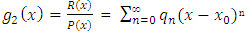 which converges for
  .Definition 2.4: Frobenius method of solving differential equation is a method that assumes that
  is a regular singular point of the differential equation.
 | (7) |
The Frobenius series of the form 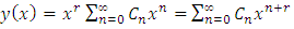 can be used to solve the differential equation (7). The parameter r must be chosen so that when the series is substituted into the differential equation the coefficient of the smallest power of x is zero. This is called the indicial equation. Also, a recursive equation for the coefficient is obtained by setting the coefficient of
  equal to zero.Definition 2.5: Let
  be the error in Simpson’s rule for a particular n i.e,
 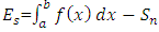 . Then if
  on
on  (for some constant k), then
 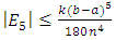 .Definition 2.6: Let
 | (8) |
A solution  of (8) is Lyapunov stable if for each
  and
and  such that if
  is a solution of (2.4) and
  then
then  for all
  .Definition 2.7: A solution
  of (8) is asymptotically stable if it is Lyapunov stable and if for every
 as
as  .Definition 2.8: Consider a real valued function
  which is continuously differentiable with
  V is said to be
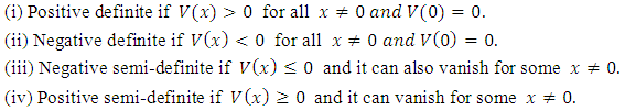 Definition 2.9: Let the origin
  be an equilibrium point for
  . Let
. Let  be a continuously differentiable function such that,
  and
and  ,
,  then
then  is stable. Moreover if
  then
then  is asymptotically stable.Corollary 2.10: Let
  be an equilibrium point of
  . Let
. Let  be a
be a  positive definite function containing the origin
  such that
  in D. Let
  and suppose that no solution can stay identically in S, other than the trivial solution
  then the origin is asymptotically stable.
2.2. Results and Discussion
2.2.1. Numerical Integration Approach
We consider a differential equation of the form | (9) |
where  Then equation (9) becomes
 | (10) |
Assume that equation (6) has a solution of the form | (11) |
Finding the derivative of  term by term gives
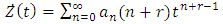 | (12) |
 | (13) |
Substituting for  and
and  in equation (10) we have,
 | (14) |
When  respectively we have
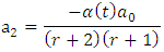
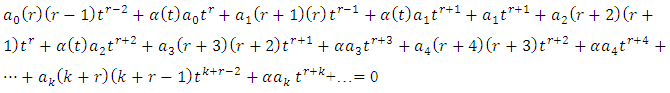 For a power series to vanish identically over the interval, the coefficient must be zero.For
 | (15) |
 Hence
Hence  = integer.For
  we have
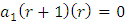 | (16) |
When  , then
 in (15) implies that
  is intermediateFor
  we have
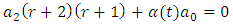 | (17) |
 | (18) |
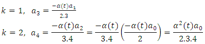
For the general term  , we have
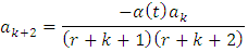 | (19) |
which gives | (20) |
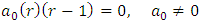
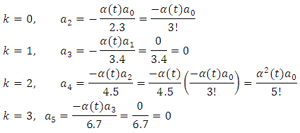
From the indicial equation  implies that
  is intermediate.From equation (20)
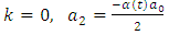
 Hence, one solution is
 | (21) |
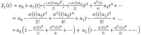 | (22) |
Since  and
and  are arbitrary constants, we have
 | (23) |
Similarly when 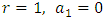
 Then
Then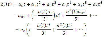 | (24) |
Since  is an arbitrary constant, we have that
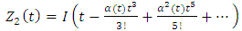 | (25) |
Hence, the general solution is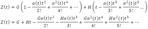 | (26) |
Since  then
then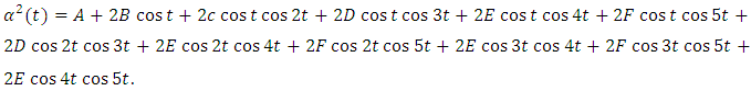 | (27) |
Let Then,
Then,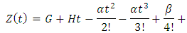 | (28) |
 | (29) |
Applying Simpson’s Integration formula on  with step size
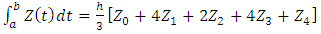 | (30) |
Let  be the interval then,
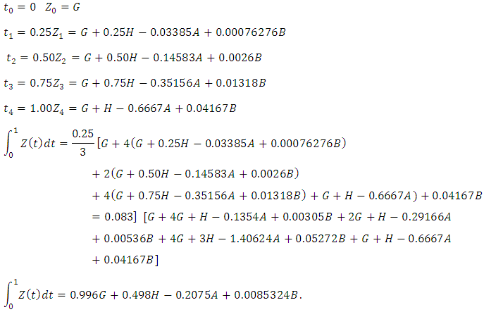 | (31) |
2.2.2. Stability Analysis
Consider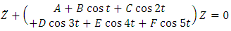 | (32) |
Let  The first equivalent systems of (32) is
 | (33) |
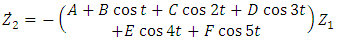 | (34) |
(33) and (34) can be written as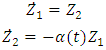 where
where  In matrix form we have
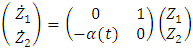 | (35) |
(35) can be written as  where A is the matrix.For the characteristics polynomial
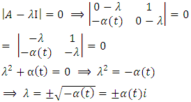 | (36) |
Hence the general solution is | (37) |
which can be written as | (38) |
Equation (38) shows that solution of Hill’s equation is periodic with respect to the independent parameters.
2.2.3. Lyapunov Direct Method
Consider the equation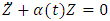 | (39) |
At fixed point  Using
Using 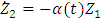 we have
  Hence at fixed point we have
  as the only equilibrium point of the system.For the Lyapunov function, we multiply equation (39) by
  which gives
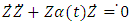 | (40) |
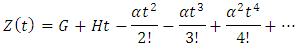
Integrating equation (40) we have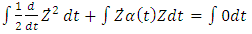 | (41) |
which gives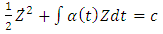 | (42) |
The energy function 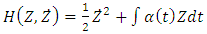 But
But  Hence the Lyapunov function is given by
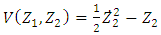 | (43) |
Applying definition (2.9) to equation (43) we have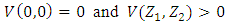 Differentiating equation (43) we have
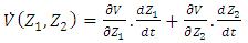 | (44) |
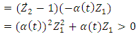 | (45) |
Hence the equilibrium point is unstable.
2.2.4. Numerical Solution of Hill’s Equation
 Define a function that determines a vector of derivative values at any solution point (t,Y):
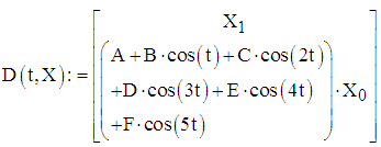 Define additional arguments for the ODE solver:
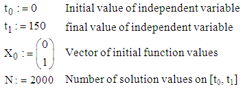 Solution matrix:
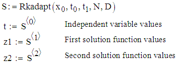
Table 1. Table of values for the independent variables
 |
| |
|
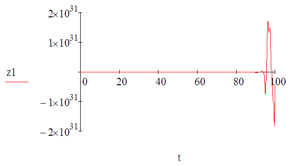 | Figure 1. The relation between first solution function values and independent variable values |
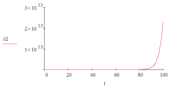
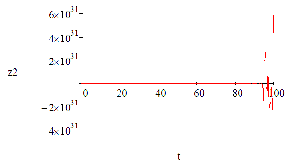 | Figure 2. The relation between second solution function values and independent variable values |
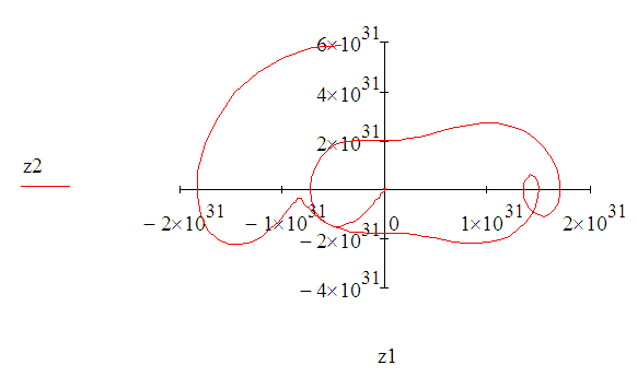 | Figure 3. Phase portrait of Hill’s equation showing instability of the solution as a spiral source |

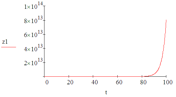 | Figure 4. The relation between the first solution function values and the independent variable values |
 | Figure 5. The relation between the second solution function values and the independent variable values |
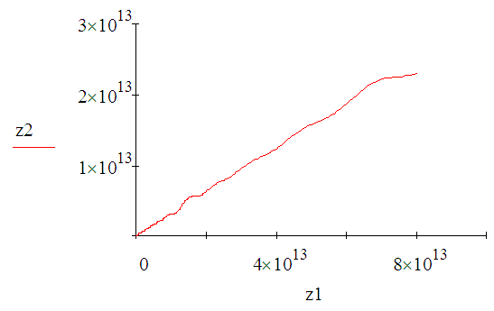 | Figure 6. The relation between first solution function values and second solution function values showing instability of Hill’s equation |

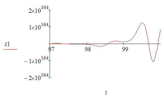 | Figure 7. Trajectory profile of first solution function values and independent variable values |
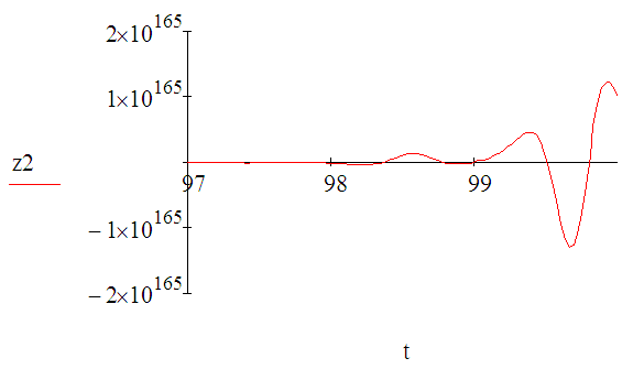 | Figure 8. Trajectory profile of second solution function values and independent variable values |
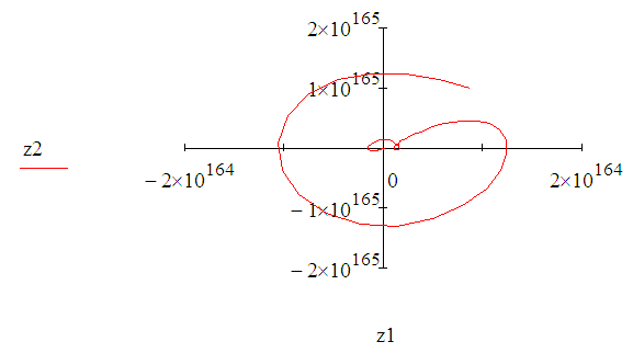 | Figure 9. Phase portrait of Hill’s equation of first solution function values and second solution function values showing instability around the origin |
3. Conclusions
From our result, it was observed that regions of instability were basically around the equilibrium point and stable otherwise.We also observed that this region of instability remained radially unbounded. Although, the total derivative existed, the region is unbounded, which implies that the existence of total derivative does not necessarily implied boundedness using Lyapunov methods.
ACKNOWLEDGEMENTS
The authors wishes to express their profound gratitude to the editor of American Journal of Computational and Applied Mathematics for providing a platform in which this paper was acknowledged and accepted.
References
| [1] | Altshaller, 1996, Robust Stability of Hill’s Equation with a delay term, Siam Journal on Control, 6(8), 25-27. |
| [2] | Chen, 2004, Basic Theory and Methodology of Lyapunov Stability, Orbital Stability and input output Stability for non-Linear System, Encyclopedia of RF and microwave engineering, Wiley, New York, 22(24), 4881-4896. |
| [3] | Langmuir and Irving, 1918, The adsorption of gases on plane surface of glass, mica and platinum. Journal of the American Chemical Society 40(9), 1361-1403. |
| [4] | Eze E.O. and Aja R.O., 2014, On Application of Lyqpunov and Yoshizawa’s Theorem on Stability, Asymptotic Stability, Boundedness and Periodicity of Solutions of Duffing Equation. Asian Journal of Applied Sciences 2(6), 630-635. |
| [5] | Grigorvan, 2013, Boundedness and Stability criteria for Linear Ordinary Differential Equations of the second order, Russian Mathematics Journal, 57(12), 8-15. |
| [6] | Franco C.A. and Collabo J., 2017, Comparison on sufficient conditions for the stability of Hill’s equation. An Arnold’s Tongue Approach, Applied Mathematics, 8, 1481-1514. |
| [7] | Raftoul Y.N., 1991, Boundedness in Non-Linear Differential Equations, Journal of Mathematics Subject Classification, 3(16), 12-14. |
| [8] | Rand R., 1969, Stability of Hill’s Equation for four independent parameters using Floquent theory and perturbations, Journal of Applied Mathematics, 4(7), 885-886. |
| [9] | Sell G.R., 1964, Boundedness of solutions of ordinary differential equations and lyapunov functions, Journal of Analysis and Applications Mathematics 3(2), 477-490. |
| [10] | Klotter K. and Kotowski G, 1967, Uber die Stabilitat der Losungen Hillscher Differentialgleichungen mit drei unabhangigen Parametern, Zeitschrift fur angewandte Mathemalik und Mechanik, 2, 1-25. |
| [11] | Zhang, 2011, Positive periodic solutions of Hill’s equation, Advancenon Linear Studies. 6(10), 57-67. |
| [12] | Oyesanya M.O, and Nwamba J.I., 2013, Stability Analysis of Damped Cubic-Quintic Duffing Oscillator, World Journal of Mechanics 3, 43-57. |
| [13] | Hill G, W., 1886, On the part of the motion of lunar pedigree which is a function of the mean motions of the sun and moon, Acta math 8 (1), 1-36. |
| [14] | Eze E.O., Ukeje E. and Ogbu H.M., 2015, The stable, bounded and periodic solutions in a non- linear second order differential equation, American Journal of Engineering research, 4(8), 14-18. |

 Abstract
 Reference
 Full-Text PDF
 Full-text HTML