Subhash Bagui1, K. L. Mehra2
1Department of Mathematics and Statistics, The University of West Florida, Pensacola, FL, United States
2Department of Mathematical and Statistical Sciences, University of Alberta, Edmonton, AB, Canada
Correspondence to: Subhash Bagui, Department of Mathematics and Statistics, The University of West Florida, Pensacola, FL, United States.
| Email: |  |
Copyright © 2019 The Author(s). Published by Scientific & Academic Publishing.
This work is licensed under the Creative Commons Attribution International License (CC BY).
http://creativecommons.org/licenses/by/4.0/

Abstract
This paper offers four different methods of proof of the convergence of negative binomial NB(n, p) distribution to a normal distribution, as  . All these methods of proof may not be available together in a book or in a single paper in literature. The reader should find the presentation enlightening and worthwhile from a pedagogical viewpoint. The article should of interest to teachers and undergraduate seniors in probability and statistics courses.
Keywords:
Negative binomial distribution, Central limit theorem, Moment generating function, Ratio method, Stirling’s approximations
Cite this paper: Subhash Bagui, K. L. Mehra, On the Convergence of Negative Binomial Distribution, American Journal of Mathematics and Statistics, Vol. 9 No. 1, 2019, pp. 44-50. doi: 10.5923/j.ajms.20190901.06.
1. Introduction
The negative binomial (NB) distribution was first initiated by Pascal (1679), although its earliest concrete formulation and introduction was due to Montmort (1741); see Todhunter (1865). Montmort derived the distribution of number of tosses of a coin required to obtain a specified number of heads. Student (1907) in an empirical study employed NB to model countings on haemocytometer data. Bartko (1961) published an excellent review article on many aspects of the NB distribution. The NB is an often used distribution in statistical modeling. The inverse binomial sampling scheme is modeled with NB distribution. This scheme is described as: in an infinite sequence of independent Bernoulli trials continue to select items until a fixed number of successes (or failures) are captured. For example, suppose we are conducting a wildlife survey and wanting to catch n of a certain type of restricted birds. In the sampling process we capture birds at random until we have bagged n of these restricted birds (and an unknown random number of other types of birds). Thus, the resulting sample size would be more than n. The NB models the distribution of either the resulting total sample size or the unknown random number of other types of birds. Thus, there are a couple of variations of the NB distribution. The first version deals with the total number of trials (say,  ) necessary to obtain n successes. With this version, the probability mass function of
  is given by
 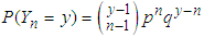 , for integer
  . Here p is the probability of success and
  is the probability of failure, with
  . If we let
  denote the number of failures before the nth success, then
 . The second version counts the number of failures before the nth success. In this version, the probability mass function of
  is given by
 | (1.1) |
It is well known that the mean of  is
is 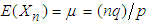 and the variance of
  is
is 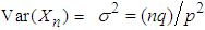 . A little algebra shows that
  . Thus, the variance is always larger than the mean for NB distribution. For the data which points to a larger variance than the mean, the Poisson distribution is unsuitable for modeling as it requires the mean and variance to be equal. In such cases, the negative binomial seems more suitable. The NB distribution has become increasingly popular as a flexible alternative to the Poisson, especially when the underlying variance seems greater than the mean and when independence of the counts is also doubtful. Among others, Arbous and Kerrich (1951), Greenwood and Yule (1920), and Kemp (1970) have applied NB to model accident statistics. Furry (1937) and Kendall (1949) have shown its applications in birth-and-death processes. For more applications see Johnson et al. (1993) and also Feller (1957). Relationship with Poisson distribution.Suppose
  follows Poisson distribution with
  following a Gamma
  ; then
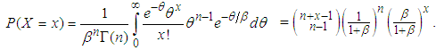 So the marginal distribution of X is negative binomial with parameters n and
  . This result was due to Greenwood and Yule (1920). They used it to model “accident proneness”. The parameter
  is the expected number of accidents for an individual, which is presumed to vary from person to person. Another important formulation is due to Luders (1934) and Quenouille (1949). In this formulation the NB arises as the distribution of the sum of N independent random variables each having the same logarithmic distribution and N having a Poisson distribution. This has application in entomology where the counts of larvae over the plots in a field are observed. The larvae are hatched from egg masses which appear at random over the field. If the number of egg masses on a plot follow a Poisson distribution and the survivors from the egg masses follow a Logarithmic distribution, then the resulting distribution of larvae on plots will be a Negative Binomial (See Gurland 1959). For various methods of approximating the NB probability, see Bartko (1965). It is well-known that as n increases indefinitely, the NB converges to a normal distribution. Accordingly, in statistical practice the NB probabilities are approximated using the appropriate normal density for large n. There are multiple ways one can show the convergence of the NB to the normal. But all these proofs may be not be found together in a single book or an article. The main aim of this article is to the present four different methods of proof of this convergence, as
  . The first proof is based on the well-known Stirling’s formula, and the other three methods are the Ratio method, the Method of Moment Generating Functions (mgf’s), and lastly that of the Central Limit Theorem. These contrasting methods of proof are useful from a pedagogical standpoint. Bagui and Mehra (1917) dealt with similar proofs for showing the convergence of Binomial to the limiting normal, as
  .The paper is organized as follows: In Section 2, we list some preliminary results that will be used in the subsequent sections for proving these convergences. The details of various poofs of convergence are provided in Section 3. Some concluding remarks are given in Section 4.
2. Preliminaries
In this section we state a few useful definitions, formulas, Lemmas, and Theorems which we shall employ in detailing a number of proofs in Section 3. Formula 2.1. For large n, the Stirling’s formula for approximating  is given by
 | (2.1) |
( stands for “approximately equals to”, in the above sense, for large n) Formula 2.2. The following equations hold:
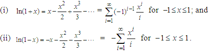 Definition 2.1. Let X be a random variable. The moment generating function (mgf) of the r.v. X is defined by
 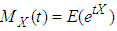 provided it is finite for all
  , for some
  .We say then that the mgf
  of X exists. If it exists, it is associated with a unique distribution. That is, there is a one-to-one correspondence between the pdf’s (or pmf’s) of X and the above defined mgf’s. Lemma 2.1. Let Z be a random variable with density
 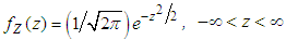 ; that is, the r.v.
  , the standard normal distribution. Then the mgf of Z is given by
 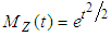 .Proof. From the above definition, the mgf of Z evaluates to
 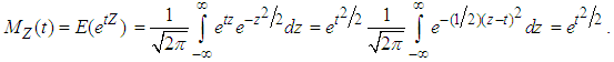 Lemma 2.2. Suppose
  is a sequence of real numbers such that
  . Then
 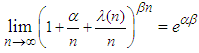 , as long as
  and
and  do not depend on n. Theorem 2.1. Suppose
  is a sequence of r.v’s with mgf’s
  for
for  and
and  . Suppose the r.v. X has mgf
  for
for  . If
. If 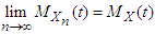 for
for  , then
  , as
, as  . (The symbolization
  means that the distribution of the r.v.
  converges to the distribution of the r.v. X, as
  ).Theorem 2.2. Let
  be a random sample of independent and identically distributed observations from a population that has a finite mean
  and a finite variance
  . Define
  and
and  . Then
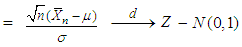 , the standard normal distribution, as
  . Theorem 2.2 is often referred to as the basic Central Limit Theorem (CLT). Big
  and Small
  notationsThe Big
  notation
  implies that the ratio
  stays bounded, as
  ; that is, there exists a positive constant
  such that
  for all n, however large the n may be. For example, if
  , as
, as  ,
,  implies that
  at the same or higher rate than that of
  . The small
  notation
  implies that the ratio
  , as
, as  ; that is, given an
  , however small, there exists an
  such that
  for all
  . Here for example, if
  , as
, as  ,
,  implies that
  at a higher rate than that of
  .
.
3. Multiple Proofs
In this section, we offer four different methods of proof for showing the convergence of negative binomial to a normal distribution, as  .
.
3.1. Stirling Approximation Formula Method
First we rewrite the negative binomial pmf given in (1.1) as 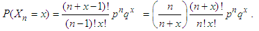 | (3.1) |
Now substitute Stirling’s approximation formula given by (2.1) in (3.1). After some algebraic simplifications, we have 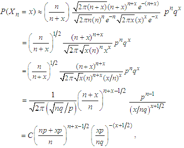 | (3.2) |
where 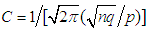 . Taking natural logarithms on both sides of (3.2), we get
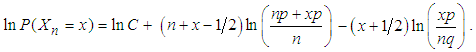 | (3.3) |
Note now that the mean  and variance
  of the NB(n, p) r.v. are given by
  and
and  , respectively. Suppose we set
  and
and  . The terms in the last equation lead to:
  , so that
 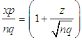 , and
, and 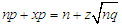 , so that
 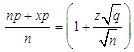 . Using the these simplifications we re-write (3.3) as
 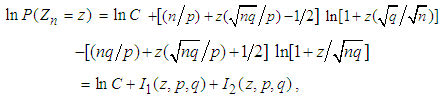 | (3.4) |
where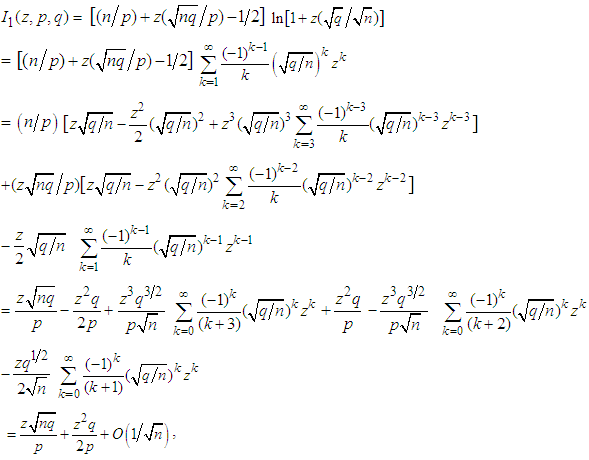 | (3.5) |
where the last order term  follows since the absolute values of the three infinite sums above can be shown to remain bounded, as
  , by applying Formulas 2.2 to each of them individually. Similarly,
 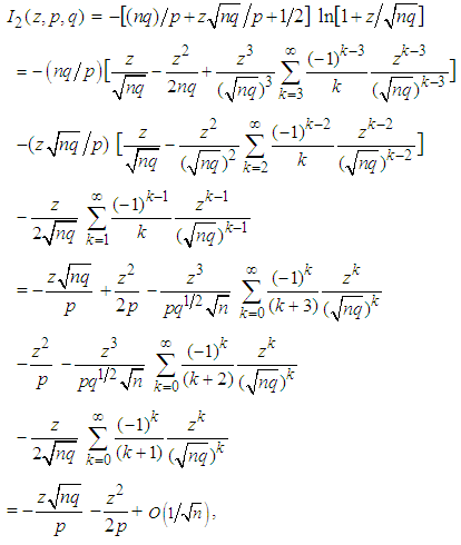 | (3.6) |
the last order term  in (3.6) following again by an application of Formulas 2.2, as done for (3.5) above.Now substituting (3.5) and (3.6) in (3.4), we have
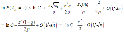 | (3.7) |
Hence, for large n, from (3.7) we get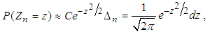 | (3.8) |
where 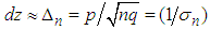 . The above equation (3.8) may also be written as
 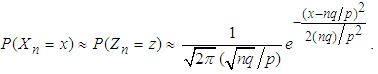 | (3.9) |
This completes the proof.
3.2. The Ratio Method [5]
The ratio method uses the ratio of two successive probability terms of the pmf. The ratio of two consecutive probability terms of the negative binomial pmf given in (1.1) is leads to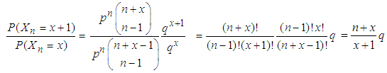 | (3.10) |
Let 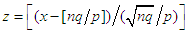 , so that
 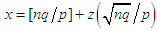 ; substituting this expression for x into (3.10), we obtain the equation
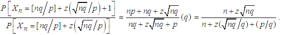 | (3.11) |
By setting 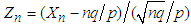 and
and  , we can rewrite (3.11) as
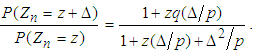 | (3.12) |
Now assume that there exists a smooth pdf  such that for large n,
 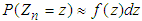 and therefore
 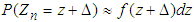 . Under this broad assumption, the left hand side of (3.12) can be rewritten as
 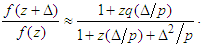 | (3.13) |
Upon taking logarithms on both sides of (3.13), dividing by  and taking limits as
  , or equivalently
  , we have
 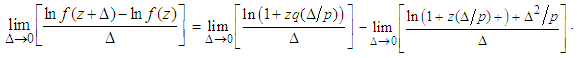 | (3.14) |
We simplify right hand side of (3.14) by applying L’Hopitals rule. Since the left hand side of (3.14) is evidently the derivative of  , as a consequence we obtain the following differential equation
 | (3.15) |
Integrating on both sides of equation (3.15) with respect to  we obtain
  , where c is the constant of integration. We can rewrite this equation as
  with
with  to make
  ,
,  , a valid density. We can conclude thus that the r.v.
  converges in distribution, as
  , to a standard normal
  r.v., or equivalently, that the negative-binomial
  r.v.
r.v.  follows approximately, for large n, the normal distribution with mean
  and
and  as the variance.
3.3. The MGF Method [4]
Let  be a negative binomial r.v. with pmf given in (1.1). Then the mgf of
  is derived as
  | (3.16) |
Let  . The mgf of
  then evaluates to
 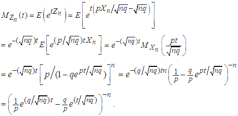 | (3.17) |
The Taylor series expansion for  gives us
 | (3.18) |
where the sequence  lies between 0 and
  and
and  as
as  . Similarly, we obtain
 | (3.19) |
where the sequence  here lies between 0 and
  and
and  as
as  .Substituting equations (3.18) and (3.19) in the last expression for
  in (3.17), after some algebraic simplifications, we have
 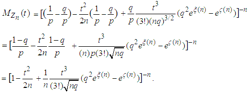 | (3.20) |
The preceding equation (3.20) may be written as 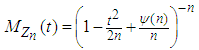 , where
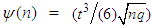
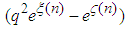 . Since both
  as
as  , it implies that
  for every fixed t . Hence, by Lemma 2.2 we have
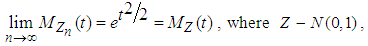 | (3.21) |
for all real t. Hence, by Theorems 2.1, we can conclude that the r.v. 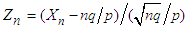 has the limiting standard normal distribution, as
  . Alternatively, we can state that the NB r.v.
  has approximately a normal distribution with mean
  and variance
  , for large n.
3.4. The CLT Techniques
Consider an infinite sequence of Bernoulli trials with success probability p,  , and failure probability
  Define the r.v. Y to be the number of failures before the first success. Then Y is said to have the Geometric distribution with parameter p. The pmf of Y can be stated as
 | (3.4.1) |
Let  be a sequence of independent and identically distributed r.v.’s from the above Geometric distribution. Define
  . Then
  denotes total number of failures before the nth success. The sum
  can be easily seen to have the negative-binomial distribution with parameters n and p. We can verify it by the mgf technique: The mgf of each
  is
is  , so that the mgf of
  is obtained as
  . This is exactly the mgf of the negative-binomial NB(n, p) r.v. derived directly in (3.16). Hence,
  follows a negative-binomial with parameters n and p. Thus, the negative binomial r.v.
  ca be viewed as the sum of n i.i.d. Geometric r.v.’s,
  , with mean
  and variance
  . Clearly therefore, the mean of
  is
is  and variance
  . Accordingly, by the CLT Theorem 2.2, we can conclude that
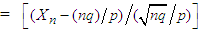
 , as
, as  or equivalently, that the r.v.
  follows approximately the normal distribution with mean
  and variance
  for large n.
4. Concluding Remarks
This article offers four different methods of proof for the convergence of negative-binomial NB(n, p) distribution to a limiting normal distribution. The first one is due to DeMoivre which uses Stirling’s Approximation formula. The second one is the Ratio Method which is based on and utilizes the ratio of two successive probability terms of the pmf and, thereby, circumvents the use of Stirling’s approximation formula. The method requires only a basic knowledge of Calculus, viz., limits, derivatives, Taylor series expansions and simple integration, along with basic probability concepts. This method also makes a broad assumption which is not always verifiable. Accordingly, the method - strictly speaking - may be regarded only as a technique rather than a complete proof. The other two methods are, respectively, the MGF method based on Laplace transforms and lastly that of the Central Limit Theorems based on Fourier transforms and the complex analysis, [3]. This article may serve as a useful teaching reference paper. The contents of this article should be of pedagogical interest to teachers, and can be discussed in senior level probability courses. It should be of reading interest for undergraduate students in probability or mathematical statistics. The teachers may gainfully assign these different methods to students as class projects.
ACKNOWLEDGEMENTS
The authors would like to thank an anonymous referee for careful reading and constructive suggestions on the earlier version of the paper.
References
| [1] | Arbous, A. G. and Kerrich, J. E. (1951). Accident statistics and the concept of accident proneness. Biometrics, 7, 340-432. |
| [2] | Bagui, S. C., Bagui, S S., and Hemasinha, R. (1913). Nonrigorous proofs of Stirling’s formula, Mathematics and Computer Education, 47, 115-125. |
| [3] | Bagui, S. C. and Mehra, K. L. (1917). Convergence of Binomial to Normal: Multiple proofs, International Mathematical Forum, 12, 399-422. |
| [4] | Bagui, S. C. and Mehra, K. L. (1916). Convergence of Binomial, Poisson, Negative Binomial and Gamma to normal distribution: Moment generating functions technique, American Journal of Mathematics and Statistics, 6, 115-121. |
| [5] | Bagui, S. C. and Mehra, K. L. (1917). Convergence of known distributions to limiting normal or non-normal distributions: An Elementary ratio technique, The American Statistician, 71(3), 265-271. |
| [6] | Bartko, J. J. (1961). The Negative binomial distribution: A review of properties and applications, Virginia Journal of Science, 12, 18-37. |
| [7] | Bartko, J. J. (1965). Approximating the Negative Binomial, Technometrics, 8(2), 345-350. Feller, W., (1957). An introduction to probability theory and its applications, 2nd edition, Wiley, New York, p. 263. |
| [8] | Furry, W. H. (1937). On fluctuation phenomena in the passage of high energy electrons through lead, Physical Review, 52, 569-581. |
| [9] | Greenwood, M. and Yule, G. U. (1920). An inquiry into the nature of frequency distributions representative of multiple happenings with particular reference to the occurrence of multiple attacks of disease or of repeated accidents, Journal of the Royal Statistical Society, A, 83, 255-279. |
| [10] | Gurland, John (1959). Some applications of the negative binomial and other contagious distributions, American Journal of Public Health, 49(10), 1388-1389. |
| [11] | Johnson, N. L., Kotz, S., and Kemp, A. W. (1993). Univariate Discrete Distributions, Wiley, New York. |
| [12] | Kemp, A. W. (1970). “Accident proneness” and discrete distribution theory, Random counts in Scientific work, 2: Random counts in Biomedical and Social Sciences, G. P. Patil (editor), 41-65. University Park: Pennsylvania State University Press. |
| [13] | Kendall, D. G. (1949). Stochastic processes and population growth, Journal of the Royal Statistical Society, B, 11, 230-282. |
| [14] | Luders, R. (1934). Die statistik der seltenen ereignisse, Biometrika, 26, 108-128. Montmort, P. R. (1741). Essai d’analyse sur les jeux de hazards. Pascal, B. (1679). Varia opera Mathematica D. Petri de Fermat: Tolossae. |
| [15] | Quenouille, M. H. (1949). A relation between the logarithmic, Poisson, and negative binomial series, Biometrics, 5, 162-164. |
| [16] | Student (1919). On the error of counting with a haemocytometer, Biometrika, 5, 351-360. |
| [17] | Todhunter, I., (1865). A history of the mathematical theory of probability from the time of Pascal to that of Laplace, MacMillan and Co, p.97. |

 Abstract
 Reference
 Full-Text PDF
 Full-text HTML