Tesfalem Eyob1, Rama Shanker1, Kamlesh Kumar Shukla1, Tekie Asehun Leonida2
1Department of Statistics, College of Science, Eritrea Institute of Technology, Asmara, Eritrea
2Department of Applied Mathematics, University of Twente, The Netherlands
Correspondence to: Tesfalem Eyob, Department of Statistics, College of Science, Eritrea Institute of Technology, Asmara, Eritrea.
| Email: |  |
Copyright © 2019 The Author(s). Published by Scientific & Academic Publishing.
This work is licensed under the Creative Commons Attribution International License (CC BY).
http://creativecommons.org/licenses/by/4.0/

Abstract
This paper proposes a three-parameter weighted quasi Akash distribution (WQAD) which includes two-parameter weighted Akash, quasi Akash and gamma distributions and one parameter Akash distribution as special cases. Its raw moments and central moments have been obtained. The moment based measures including coefficient of variation, skewness, kurtosis and index of dispersion have been discussed. The statistical properties including hazard rate function, mean residual life function and stochastic ordering have been explained. Maximum likelihood estimation has been discussed for estimating the parameters of the distribution. Finally, applications of the distribution have been explained with three examples of observed real lifetime datasets from engineering.
Keywords:
Quasi Akash distribution, Moments, Statistical properties, Maximum Likelihood estimation, Goodness of fit
Cite this paper: Tesfalem Eyob, Rama Shanker, Kamlesh Kumar Shukla, Tekie Asehun Leonida, Weighted Quasi Akash Distribution: Properties and Applications, American Journal of Mathematics and Statistics, Vol. 9 No. 1, 2019, pp. 30-43. doi: 10.5923/j.ajms.20190901.05.
1. Introduction
Let the original observation  comes from a distribution having probability density function (pdf)
  , where
  may be a parameter vector and the observation x is recorded according to a probability re-weighted by weight function
  ,
,  being a new parameter vector, then x comes from a distribution having pdf
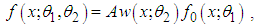 | (1.1) |
where A is a normalizing constant. Note that such types of distribution are known as weighted distributions. The weighted distributions with weight function  are called length biased distributions or simple size-biased distributions. Patil and Rao (1977, 1978) have examined some general probability models leading to weighted probability distributions, discussed their applications and showed the occurrence of
  in a natural way in problems relating to sampling.The study of weighted distributions are useful in distribution theory because it provides a new understanding of the existing standard probability distributions and it provides methods for extending existing standard probability distributions for modeling lifetime data due to introduction of additional parameter in the model which creates flexibility in their nature. Weighted distributions occur in modeling clustered sampling, heterogeneity, and extraneous variation in the dataset.The concept of weighted distributions were firstly introduced by Fisher (1934) to model ascertainment biases which were later formulized by Rao (1965) in a unifying theory for problems where the observations fall in non-experimental, non-replicated and non-random manner. When observations are recorded by an investigator in the nature according to certain stochastic model, the distribution of the recorded observations will not have the original distribution unless every observation is given an equal chance of being recorded.Shanker (2016) proposed a two-parameter quasi Akash distribution (QAD) with parameters
  and
and  defined by its probability density function (pdf) and cumulative density function (cdf)
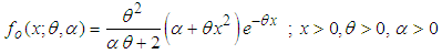 | (1.2) |
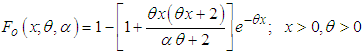 | (1.3) |
It can be easily verified that at  , (1.1) reduces to gamma
  distribution and at
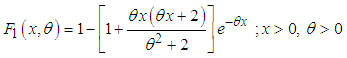
  , (1.2) reduces to Akash distribution introduced by Shanker (2015) having pdf and cdf
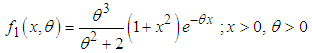 | (1.4) |
 | (1.5) |
The rth moment about origin,  , of QAD obtained by Shanker (2016) is
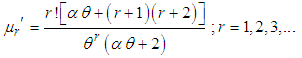 | (1.6) |
The first four moments about origin and the central moments of QAD are obtained as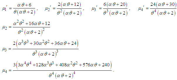 In the present paper, a three - parameter weighted quasi Akash distribution which includes Akash distribution, weighted Akash distribution, quasi Akash distribution and gamma distribution as particular cases, has been proposed and discussed. Its raw moments and central moments, coefficient of variation, skewness, kurtosis and index of dispersion have been obtained. The hazard rate function and the mean residual life function of the distribution have been derived and their behaviors have been studied for varying values of the parameters. The estimation of its parameters has been discussed using the method of maximum likelihood. Finally, the goodness of fit of the distribution have been explained through three real lifetime data from engineering and the fit has been compared with one parameter Akash distribution and Lindley distribution introduced by Lindley (1958), two-parameter quasi Akash distribution, and three-parameter weighted Lindley distribution proposed by Shanker et al (2017).
2. Weighted Quasi Akash Distribution
Using (1.1) and (1.2) with weight function 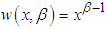 , a three - parameter weighted quasi Akash distribution (WQAD) having parameters
  , and
, and  can be defined by its pdf
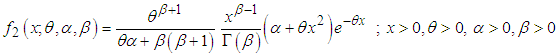 | (2.1) |
where  are shape parameters and
  is a scale parameter. It can be easily verified that the weighted Akash distribution (WAD) with parameters
  introduced by Shanker and Shukla (2016), quasi Akash distribution (QAD) with parameters
  proposed by Shanker (2016), one - parameter Akash distribution, and gamma distribution with parameters
  are particular cases of (2.1) for
 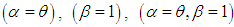 , and
, and  respectively.The corresponding cumulative distribution function of the WQAD (2.1) can be obtained as
 | (2.2) |
where  is the upper incomplete gamma function defined as
 | (2.3) |
The nature of the pdf of WQAD for varying values of the parameters has been shown graphically in figure 1. | Figure 1. The graphs of pdf of WQAD for varying values of the parameters |
The nature of the cdf of WQAD for varying values of the parameters has been shown graphically in figure 2.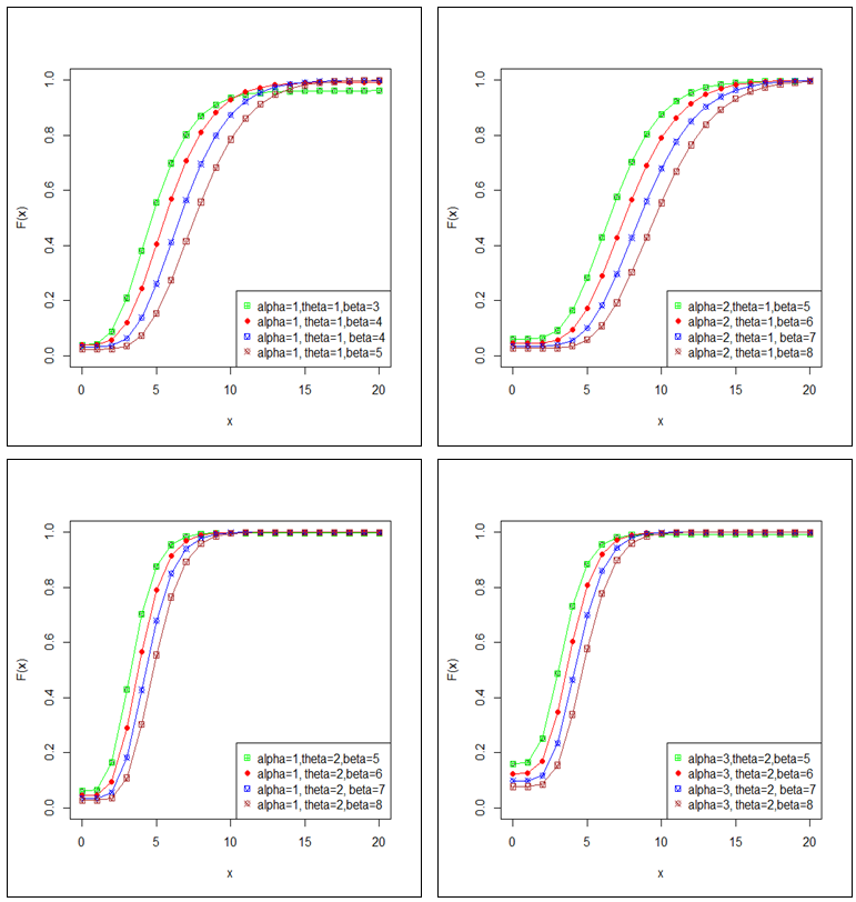 | Figure 2. The graphs of cdf of WQAD for varying values of the parameters |
3. Moments and Moments Based Measures
The  th moment about origin,
  , of WQAD can be obtained as
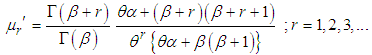 | (3.1) |
The first four moments about origin (raw moments) of WQAD are obtained as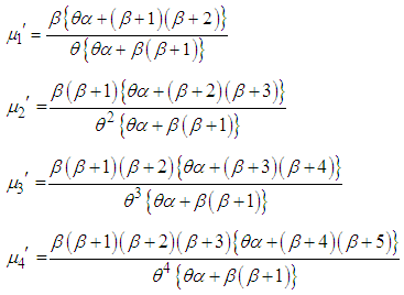 Using relationship between central moments (moments about the mean) and moments about origin, the central moments of WQAD are obtained as
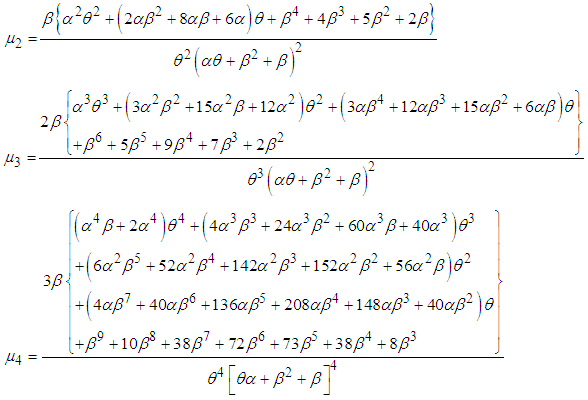 The expressions for coefficient of variation (C.V.) coefficient of skewness
  , coefficient of kurtosis
  , and index of dispersion
  of the WQAD (2.1) are thus obtained as
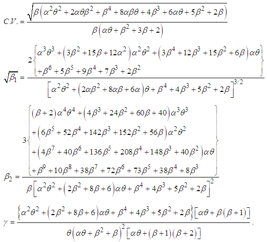 The nature of coefficient of variation, skewness, kurtosis and index of dispersion of WQAD are shown in figure 3.
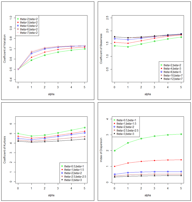 | Figure 3. Graphs of coefficient of variation, coefficient of skewness, coefficient of kurtosis and index of dispersion of WQAD for varying values of the parameters |
4. Stochastic Ordering
The stochastic ordering of positive continuous random variables is an important tool for judging their comparative behavior. A continuous random variable X is said to be smaller than a continuous random variable Y in the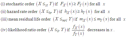 The following stochastic ordering relationships due to Shaked and Shanthikumar (1994) are well known for establishing stochastic ordering of continuous distributions
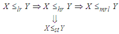 The WQAD is ordered with respect to the strongest ‘likelihood ratio’ ordering as shown in the following theorem:Theorem: Let
  and
and  . Then the following results hold true
 Proof: We have
 Now,
Now, This gives
  For
For  ,
, 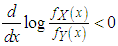 . This means that
  and hence
  ,
,  and
and  and thus (i) is verified. Similarly (ii), (iii) and (iv) can be easily verified.
5. Hazard Rate Function and Mean Residual Life Function
5.1. Hazard Rate Function
The survival (reliability) function of WQAD can be obtained as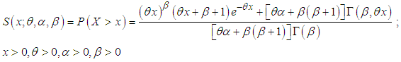 | (5.1) |
where  is the upper incomplete gamma function defined in (2.3)The hazard (or failure) rate function,
  of WQAD is thus obtained as
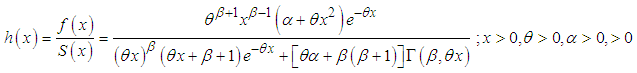 | (5.2) |
The shapes of the hazard rate function,  of the WQAD for varying values of the parameters are shown in the figure 4.
 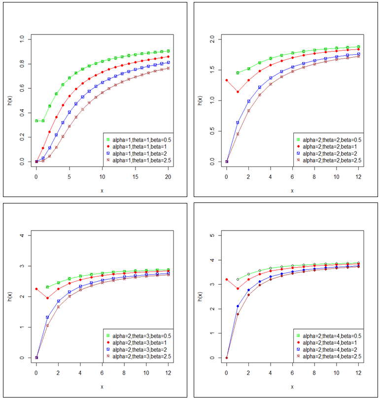 | Figure 4. The hazard rate function, h(x) of the WQAD for varying values of the parameters |
5.2. Mean Residual Life Function
The mean residual life function 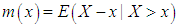 of the WQAD can be obtained as
 It can easily be verified that
  The shapes of the mean residual life function,
  of the WQAD for varying values of the parameters are shown in figure 5.
 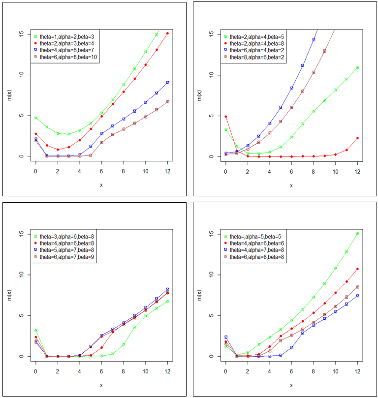 | Figure 5. The mean residual life function, m(x) of the WQAD for varying values of the parameters |
6. Maximum Likelihood Estimation of Parameters
Let 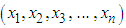 be a random sample of size n from WQAD. The likelihood function, L of WQAD is given by
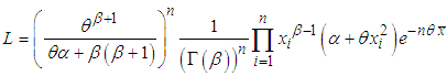 The natural log likelihood function is thus obtained as
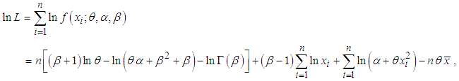 where
where  being the sample mean.The maximum likelihood estimates (MLEs)
  of parameters
  of WQAD are the solution of the following nonlinear equations
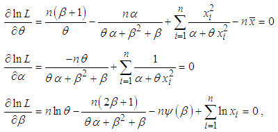 where
where 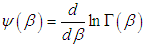 is the digamma function.These three natural log likelihood equations do not seem to be solved directly, because these equations cannot be expressed in closed forms. The (MLE’s)
  of parameters
  can be computed directly by solving the natural log likelihood equation using Newton-Raphson iteration available in R-software till sufficiently close values of
  are obtained. It can be easily proved the existence of MLE of parameters using Hessian matrix. Hessian matrix of log-likelihood function
  is the matrix of second order partial derivatives of
  with respect to parameters
  . The Hessian matrix of log-likelihood function
  can be expressed as
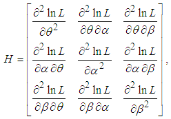 where
where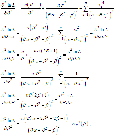 where
where  is the tri-gamma function.Now for a given stationary values of parameters, it can be easily shown that the leading principal minors of H are
 ,
,  and
and  , which means that the Hessian matrix is negative definite and hence stationary points are global maximum points.
7. Data Analysis
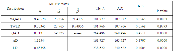
In this section three datasets from engineering has been considered for testing the goodness of fit of WQAD. The following three datasets has been considered.Data set 1: The data set represents the strength of 1.5cm glass fibers measured at the National Physical Laboratory, England. Unfortunately, the units of measurements are not given in the paper, and they are taken from Smith and Naylor (1987)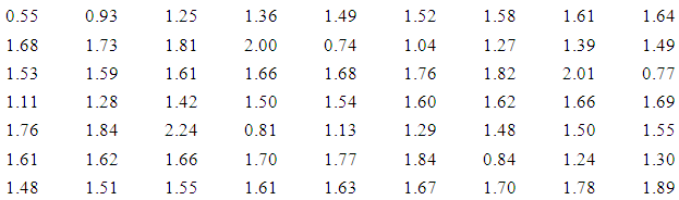 Data Set 2: This data set is the strength data of glass of the aircraft window reported by Fuller et al (1994):
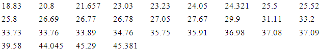 Dataset 3: A numerical example of real lifetime data has been presented to test the goodness of fit of WRD over other one parameter and two parameter life time distribution. The following data represent the tensile strength, measured in GPa, of 69 carbon fibers tested under tension at gauge lengths of 20mm, available in Bader and Priest (1982)
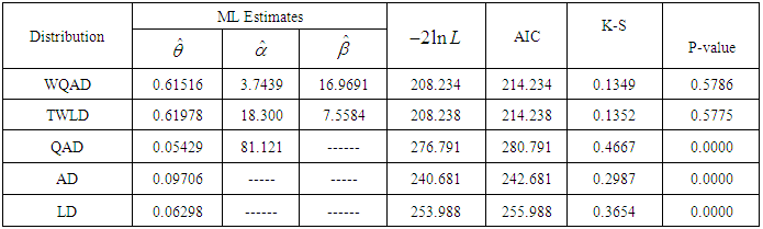
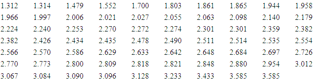 For the these three datasets, WQAD has been fitted along with one parameter Lindley distribution (LD) and Akash distribution (AD), two-parameter quasi Akash distribution (QAD) and three parameter weighted Lindley distribution (TWLD). The ML estimates, values of
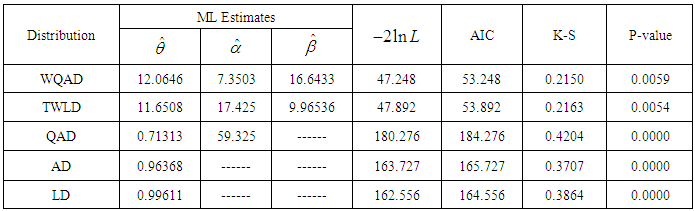
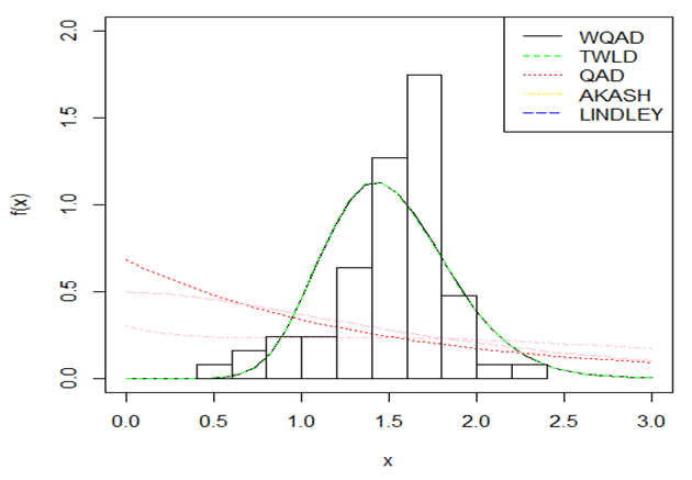
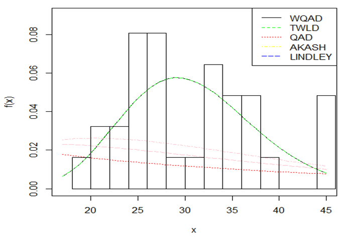
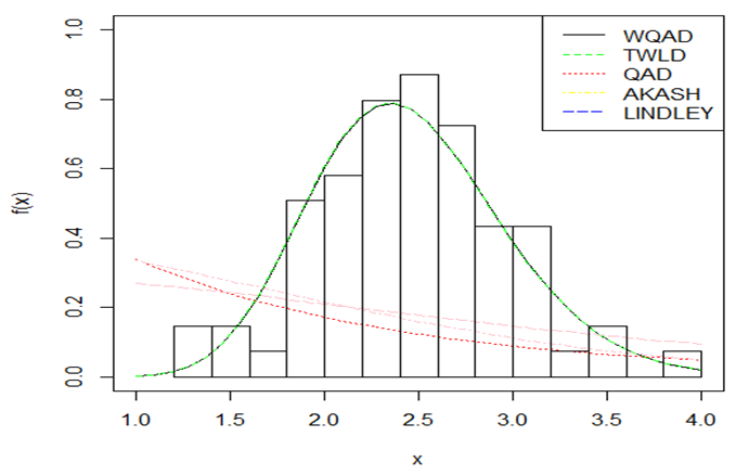
  , Akaike Information criteria (AIC), K-S statistics and p-value of the fitted distributions are presented in tables 1, 2, and 3. Also the fitted pdf plots of these distributions has been shown in figures 6, 7, and 8 The AIC and K-S Statistics are computed using the following formulae:
  and
and  , where k = the number of parameters, n = the sample size,
  is the empirical (sample) cumulative distribution function, and
  is the theoretical cumulative distribution function. The best distribution is the distribution corresponding to lower values of
  , AIC, and K-S statistics.It is obvious from the goodness of fit in the above tables and the pdf plots of fitted distributions that WQAD gives much closer fit than the three- parameter WLD, two- parameter QAD and one parameter Lindley and Akash distributions. Thus, it can be considered as an important tool for modeling real lifetime data from engineering over these distributions.
 Table 1. MLE’s, - 2ln L, AIC, K-S and p-values of the fitted distributions for dataset 1
 |
| |
|
 | Figure 6. Fitted pdf plots of the distributions for dataset 1 |
Table 2. MLE’s, - 2ln L, AIC, K-S Statistics and p-values of the fitted distributions for dataset 2
 |
| |
|
 | Figure 7. Fitted pdf plots of the distributions for dataset 2 |
Table 3. MLE’s, - 2ln L, AIC, K-S Statistics and p-values of the fitted distributions for dataset 3
 |
| |
|
 | Figure 8. Fitted pdf plots of the distributions for dataset 3 |
8. Concluding Remarks
In this paper a three - parameter weighted quasi Akash distribution (WQAD) which includes Akash distribution, weighted Akash distribution, quasi Akash distribution and gamma distribution as particular cases, has introduced and discussed. Its moments, coefficient of variation, skewness, kurtosis and index of dispersion have been obtained. The reliability properties including hazard rate function and the mean residual life function of the distribution have been derived and their behaviors have been studied for varying values of the parameters. Method of maximum likelihood has been discussed for estimating the parameters of the distribution. goodness of fit of the distribution have been explained through three real lifetime data from engineering and the fit has been compared with one parameter Akash distribution and Lindley distribution, two-parameter quasi Akash distribution, and three-parameter weighted Lindley distribution. The fit by proposed distribution has been found quite satisfactory over the considered distributions.
ACKNOWLEDGEMENTS
Authors are grateful to the editor-in-chief of the journal and anonymous reviewer for their fruitful comments which improved the quality of the paper.
References
| [1] | Bader, M.G., Priest, A. M. (1982): Statistical aspects of fiber and bundle strength in hybrid composites, In; hayashi, T., Kawata, K. Umekawa, S. (Eds), Progress in Science in Engineering Composites, ICCM-IV, Tokyo, 1129 – 1136. |
| [2] | Fisher, R.A. (1934): The effects of methods of ascertainment upon the estimation of frequencies, Ann. Eugenics, 6, 13 – 25. |
| [3] | Fuller, E.J., Frieman, S., Quinn, G., and Carter, W. (1994): Fracture mechanics approach to the design of glass aircraft windows: A case study, SPIE proc 2286, 419-430. |
| [4] | Lindley, D.V. (1958): Fiducial distributions and Bayes’ theorem, Journal of the Royal Statistical Society, Series B, 20, 102- 107. |
| [5] | Patil, G.P. and Rao, C.R. (1978): Weighted distributions and size-biased sampling with applications to wild-life populations and human families, Biometrics, 34, 179 – 189. |
| [6] | Patil, G.P. and Rao, C.R. (1977): The Weighted distributions: A survey and their applications, In applications of Statistics (Ed P.R. Krishnaiah0, 383 – 405, North Holland Publications Co., Amsterdam. |
| [7] | Shaked, M. and Shanthikumar, J.G. (1994): Stochastic Orders and Their Applications, Academic Press, New York. |
| [8] | Shanker, R. (2016): A Quasi Akash Distribution, Assam Statistical Review, 30(1), 135-160. |
| [9] | Shanker, R. (2015): Akash distribution and Its Applications, International Journal of Probability and Statistics, 4(3), 65-75. |
| [10] | Shanker, R., Shukla, K.K. (2016): Weighted Akash Distribution and Its Application to model lifetime data, International Journal of Statistics, 39(2), 1138-1147. |
| [11] | Shanker, R., Shukla, K.K., and Mishra, A. (2017): A Three- parameter weighted Lindley distribution and its applications to model survival time data, Statistics in Transition-New Series, 18 (2), 291 – 300. |
| [12] | Smith, R. L., and Naylor, J.C. (1987): A comparison of Maximum likelihood and Bayesian estimators for three parameter Weibull distribution, Applied Statistics, 36, 358-369. |

 Abstract
 Reference
 Full-Text PDF
 Full-text HTML