1. Introduction

Malaria is a mosquito- borne disease caused by a parasite called Plasmodium. This Plasmodium has four species which include Plasmodium falciparum, Plasmodium vivax, Plasmodium ovale and Plasmodium malariae. Malaria parasite is transmitted from one person to another through the bite of a female Anopheles Mosquito which require blood to nurture her eggs [1-3]. When Malaria parasites enter the blood stream of a person, they infect and destroy the red blood cells. The destruction of these essential cells leads to fever and flu-like symptoms such as chills, headache, muscle aches, tiredness, nausea, vomiting and diarrhea. Malaria, when not treated, can lead to coma and hence death [4-6]. According to World Health Organization (WHO), Center for Disease Control and Prevention (CDCP), Roll Back Malaria Partnership (RBM) (2010), 3.3 billion people, half the world’s population, are at risk of Malaria; one million people die each year from Malaria; every 30 seconds a child dies from Malaria [7-11]. Also, in Africa, 91% of all Malaria death cases occur in Sub- Sahara Africa; 1 in 5 childhood deaths are caused by Malaria; 10, 000 pregnant women and 200, 000 infants die from Malaria every year [12-15]. Furthermore, one in ten infant’s deaths and 25% of deaths in children below the age of four years is attributable to Malaria in Africa [16-18]. The country records about 1858 deaths per 100, 000 population from Malaria and Malaria is responsible for 60% of patients visits to health facilities and also about 30% and 11% of childhood and adult deaths, respectively [19-21].

2. Materials and Method

In this paper, we have used the Time series data on Malaria Mortality Cases for past 20 years (1996 -2015). The mortality data were sourced from the records unit of Federal Medical Centre Asaba, Delta State, Nigeria. We have used GRETL (Gnu Regression, Econometrics and Time-series Library) software for plotting the graphs and analysis of the data set.

2.1. Box-Jenkins Arima Model

where, is time series at time t, is the proceeding time series of is the first order difference, is the second order difference of the current observation, is the current observation and is the preceding time series to in the same series.

After the appropriate differencing, the expected time series is expected to exhibit features of a stationary time series so that the appropriate ARIMA process can be used to model the remaining serial correlation in the series [8], where p is the number of auto regressive terms, d is the number of non-seasonal differences, q is the number of lagged forecast errors in the prediction equation. For a time series process , is the first order auto-regressive process and is given by;

And a first order moving average process and is given by;

Where and are coefficients of polynomial with order p and q respectively. Alternatively, the model ultimately derived may be a mixture of these processes and of higher order; in that case, a stationary ARMA process is defined by;

Where is the degree of the differencing, is independently and normally distributed residual with zero mean and constant variance for

2.2. Model Identification (Selecting an Initial Model)

We first Determine whether the series is stationary or not by considering the graph of ACF. If a graph of ACF of the time series values either cuts off fairly quickly or dies down fairly quickly, then the time series values should be considered stationary. If a graph of ACF dies down extremely slowly, then the time series values should be considered non-stationary. If the series is not stationary; it would then be converted to a stationary series by differencing. That is, the original series is replaced by a series of differences. An ARIMA model is then specified for the differenced series. Differencing is done until a plot of the data indicates the series varies about a fixed level, and the graph of ACF either cuts off fairly quickly or dies down fairly quickly. Once a stationary series has been obtained, then the form of the model to be used can be identified.

2.3. Model Estimation and Evaluation

Once a model is identified, the next stage for Box-Jenkins approach is to Estimate the parameters. In this research, the estimation of parameters was done using maximum likelihood estimation (MLE) [22-23].

2.3.1. Maximum Likelihood Estimation of ARIMA Model

For an independent and identically distributed (idd) data with marginal pdf the density function for a sample is simply the product of the marginal densities for each observation which is given as;

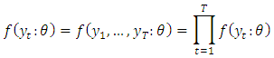The likelihood function is this joint treated as a function of the parameters given the data y;

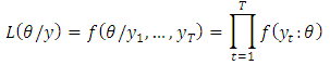The log-likelihood then as a sample form is obtained as;

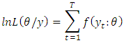For a sample from a covariance stationary time series the construction of the log-likelihood given above doesn’t work because the random variables in the sample are not independently and identically distributed. One solution is to try to determine the joint density function 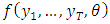directly which requires among other things variance ARIMA process. An alternative approach relies on factorization of the joint density into a series of conditional densities and the density of a set of initial values.

In order to illustrate this approach, we consider the joint density of two adjacent observations from the covariance stationary time series. The joint density can always be factored as the product of the conditional density given and the marginal density of as;

Hence for three (3) observations, the factorization becomes:

In general, the conditional marginal factorization becomes;

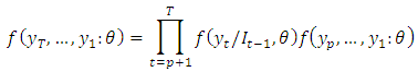Where denotes the information available at time t and denotes the initial values. The log-likelihood function may then be expressed as:

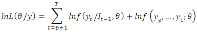The full log-likelihood function is called the exact log-likelihood. The first term is called the conditional log-likelihood and the second term is called marginal log-likelihood for the initial values.

In the maximum likelihood estimation of time series models, two types of maximum likelihood estimation (mles) may be computed. The first type is based on maximizing the conditional log-likelihood function. These estimates are called conditional MLEs and are defined by

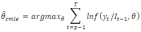The second type is based on maximizing the exact log-likelihood function. These estimates are called exact MLEs and are defined by;

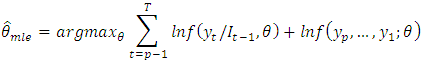For stationary models, and are consistent and have the same limiting normal distribution. In finite samples, and are generally not equal and may differ by a substantial amount if the data are close to being non-stationary.

2.4. Model Checking (Goodness of Fit)

In this step, the model must be checked for adequacy by considering the properties of the residuals whether the residuals from an ARIMA model must have the normal distribution or should be random. An overall check of the model adequacy is provided by using the Ljung-Box statistic. The test statistic Q is given as;

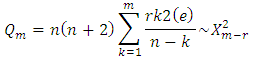where (e) is the residual autocorrelation at lag, n is the number of residual and m is the number of times lags is included in the test.

If the p-value associated with the Q statistic is small (p-value<α), then the model is considered inadequate. We then consider a new model and continue the analysis until a satisfactory model is obtained.

2.5. Forecasting

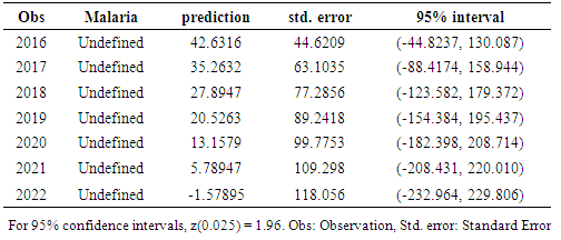
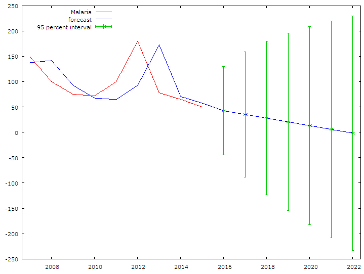
Once the model has been selected, the estimated residuals of the model is carefully examined to follow a white noise process. The parameters of the model are tested for significance and the final model estimated, then forecasting is done. Forecasting with this system is straight forward; the forecast is the expected values, evaluated at a particular point in time. Confidence intervals may also be easily derived from the standard errors of the residuals.

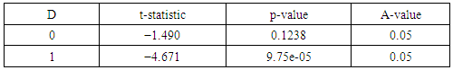
2.6. The Augmented Dickey - Fuller Test

The augmented Dickey–Fuller (ADF) test is most widely used test for checking Stationarity of a series. If d equals 0, the model becomes ARMA, which is linear stationary model. ARIMA (i.e. d > 0) is a linear non-stationary model. If the underlying time series is non-stationary, taking the difference of the series with itself predecessor to determine d makes it stationary, and then ARMA is applied onto the differenced series. A stationary process has a constant mean and variance over the time period. There are various methods available to make a time series stationary. Normally differencing techniques are used to transform a time series from a non-stationary to stationary by subtracting each datum in the series from its predecessor [8-14].

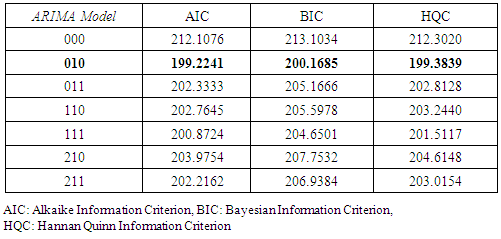
2.7. Model Identification Criteria

At the identification stage different ARIMA are formulated and tested on the data then their respective Akaike Information Criterion, Schwarz-Bayesian Information Criteria (BIC) and Hannan-Quinn Criteria (HQC) were considered and recorded. In each case, the model with the least AIC, BIC and HQC values were selected and subjected to diagnostic check to ensure that they fit well with the data [10]. The final model after estimation can be selected using a penalty function statistic such as the Akaike Information Criterion (AIC), a measure of the goodness of fit an estimated statistical model. Given a data set, several competing models may be ranked according to their AIC with one having the lowest information criterion value being the best. These information criterion judges a model by how close its fitted values, in terms of certain expected values. The criterion value assigned to a model is only meant to rank competing models and tell the best among the given alternatives. The criterion attempts to find the model that best explains the data with minimum of free parameters but also includes a penalty that is an increasing function of the number of estimated parameters.

Generally, the AIC is calculated using the relation;

where k is the number of parameters in the statistical model, and L is the maximized value of the likelihood function for the estimated model.

where is the mean square error, this implies that;

3. Results and Discussion

Malaria Mortality

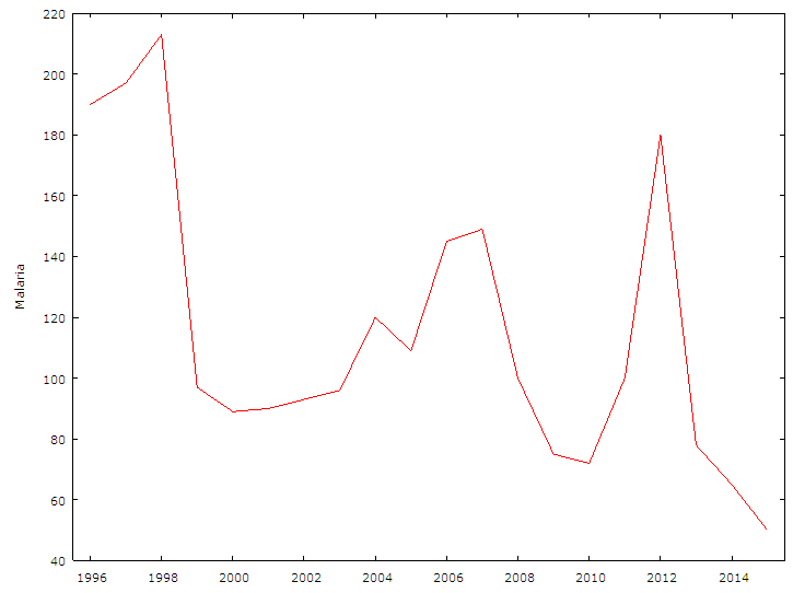Figure 1. The Graph Above is the Time Series plot for Malaria Mortality data Series

Table 1. The table below shows the Augmented Dickey-Fuller test for Stationarity of Malaria Mortality data series

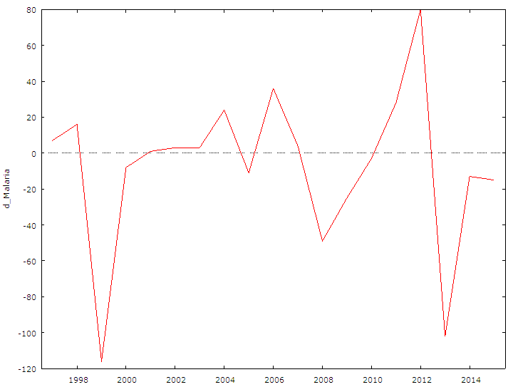Figure 2. The graph above shows the Time Series plot for differenced Malaria Mortality data series

The non Stationarity of the time series plot on Malaria Mortality data series was confirmed with the help of the augmented dickey-fuller (ADF) test on Table 1, by using first order differencing transformation, we obtained a t-statistic lesser than what was obtained at d = 0, and a p-value lesser than 5% alpha level. Thus, we select the condition that d = 1 and transform the data using first order differencing to make it stationary as seen on Figure 2.

Table 2. Table presents identification of Best ARIMA model for Malaria Mortality

Seven tentative models were entertained, and the model with the minimum AIC, BIC and HQC was chosen as the best model. ARIMA (0,1,0) was chosen as the best/ appropriate model for modeling and forecasting malaria mortality in delta state, a diagnostic check was performed using residual ACF/PACF plot at different lags and testing the significance of the correlations up to 16 lags by Q statistic and respective p-values.

3.1. Diagnostic Check on the Best Model for Malaria Mortality / Model Verification

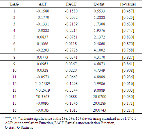
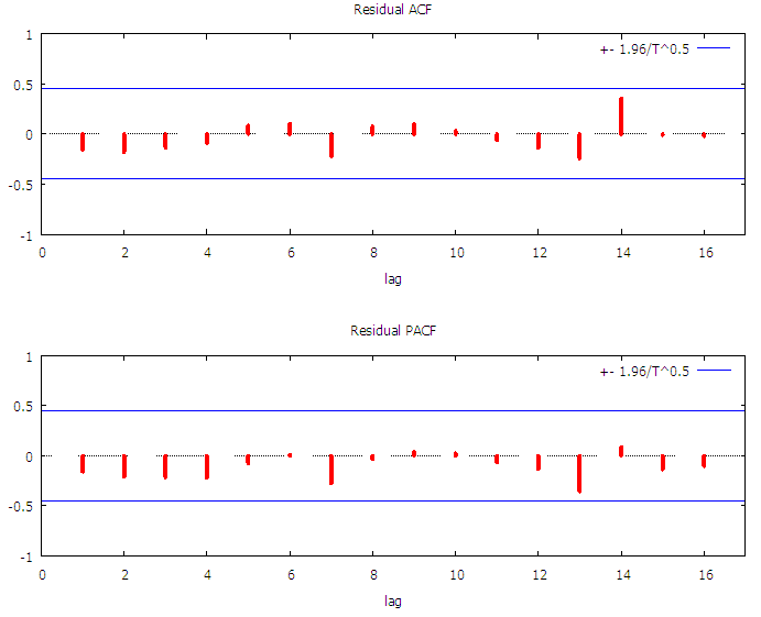Figure 3. The figure presents the Correlogram of residuals for Malaria Mortality

Figure 3 above clearly shows evidence of random walk as the values are within the bounds and undulate about zero. Hence we uphold the first order differencing.

Table 3. The table presents the residual autocorrelation function

Clearly, none of these correlations is significantly different from zero at a reasonable level. The ACF and PACF of the residuals also indicate good fit of the model. This proves that the selected ARIMA model is an appropriate model.

Table 4. The table presents the forecasting for Malaria Mortality Rate using ARIMA (0,1,0)

Figure 4. The table presents the Correlogram of residuals for Malaria Mortality

The forecast on Table 4 and Figure 4 above, suggests that malaria mortality in Delta State would be on the decrease for upcoming years.

4. Conclusions and Recommendations

Findings from this research are similar to those from [11, 12] who attempted to model malaria mortality in rural Ethiopia and South Sudan. However, in their study, Malaria mortality was seen to be on an increase [11, 12] in both south Sudan and rural Ethiopia. ARIMA (0,1,0) has been successfully used to forecast Malaria Mortality Rate in Delta State, Nigeria. Malaria Mortality was found to be on a decrease in the forecasted period. However, in order to zero mortality due to malaria from our society, government and health experts still need to put hands together to sanitize the system in terms of drugs manufacturing, bodies like NAFDAC (National Agency for Food and Drug Administration Control) needs to thoroughly monitor the drug market and ensure that drugs and food meets the necessary standards before they meet the people. There is need to sensitize the people on the use of traditional medicines and herbs.