Babalola M. Afeez1, Obubu Maxwell2, Oluwaseun A. Otekunrin3, Obiora-Ilono Happiness2
1Department of Statistics, University of Ilorin, Ilorin, Nigeria
2Department of Statistics, Nnamdi Azikiwe University, Awka, Nigeria
3Department of Statistics, University of Ibadan, Nigeria
Correspondence to: Babalola M. Afeez, Department of Statistics, University of Ilorin, Ilorin, Nigeria.
| Email: |  |
Copyright © 2018 The Author(s). Published by Scientific & Academic Publishing.
This work is licensed under the Creative Commons Attribution International License (CC BY).
http://creativecommons.org/licenses/by/4.0/

Abstract
The goal of this study is to investigate the best goodness-of-fit test among five selected normality tests under various continuous non-normal distributions using power as criteria. The tests were compared when the normal parameters are unknown and sample sizes are 10, 30, 50, 100, 300, 500 and 1000 were iterated 1000 times each with 0.01, 0.05, and 0.10 level of significance, using the Monte Carlo technique. We study the procedures based on five well-known normality tests: the Anderson–Darling, Cramer–von Mises, Shapiro–Wilk, Jarque–Bera and Chi-Square. Evidence from the simulation study reveals that the performance of the five normality test statistics varies with the level of significance, sample size and alternative distributions.
Keywords:
Normal Distributions, Shapiro-Wilk test (SW), Cramer von Misses test (CVM), Jarque-Bera test (JB), Chi-Square test (CSQ) and Anderson-Darling test (AD)
Cite this paper: Babalola M. Afeez, Obubu Maxwell, Oluwaseun A. Otekunrin, Obiora-Ilono Happiness, Selection and Validation of Comparative Study of Normality Test, American Journal of Mathematics and Statistics, Vol. 8 No. 6, 2018, pp. 190-201. doi: 10.5923/j.ajms.20180806.05.
1. Introduction
Tests of normality are statistical inference procedures design to verify that an underlying distribution of a random variable is normally distributed. The problem of testing normality is fundamental in both theoretical and empirical research. Indeed, the validity of parametric statistical inference procedures in finite samples (in the sense that their size is controlled) depends crucially on the underlying distributional assumptions. Consequently, there has been extensive focus on whether hypothesized distributions are compatible with the data. Tests of normality are particularly prevalent because the assumption of normality is quite often made in statistical analysis, e.g. in econometric studies. In this respect, the reviews by D’Agostino and Stephens (1986, Ch. 9) and Dufour et al. (1998) report nearly 40 different normality tests.However, the tests of normality are based on different characteristics of the normal distribution and the power of these tests differs depending on the nature of non-normality (Seier, 2002). And a test is said to be powerful when it has a high probability of rejecting the null hypothesis of normality when the sample under study is taken from a non-normal distribution.The effort of developing techniques to detect departures from normality was initiated by Pearson (1895) who worked on the skewness and kurtosis coefficients (Althouse et al., 1998). Tests of normality differ in the characteristics of the normal distribution they focus on, such as its skewness and kurtosis values, its distribution or characteristic function, and the linear relationship existing between the distribution of the variable and the standard normal variable, Z. The tests also differ in the level at which they compare the empirical distribution with the normal distribution, in the complexity of the test statistic and the nature of its distribution (Seier, 2002). However, Seier (2002) classified the tests of normality into four major sub-categories which are skewness and kurtosis test, empirical distribution test, regression and correlation test and other special test. Arshad et al. (2003) also categorized the tests of normality into four major categories which are tests of chi-square types, moment ratio techniques, tests based on correlation and tests based on the empirical distribution function.As it has been stated above that there are various normality tests in the literature. Some are either too simple to be powerful or too difficult to apply. Most of them are only applicable for certain situations due to various kinds of biases. But, this study is mainly focused on comparing the power of five normality tests, which are: Shapiro-Wilk test (SW), Cramer von Misses test (CVM), Jarque-Bera test (JB), Chi-Square test (CSQ) and Anderson-Darling test (AD). These formal normality tests were selected for two reasons. First, they are among the best and commonly used normality tests, Arshad et al. (2003) and Seier (2002). Second, they are available in most statistical packages, and are widely used in practice (Yap & Sim. 2011).
2. Simulation Methodology
2.1. The Normal Distribution
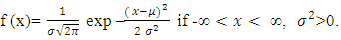
One of the most, if not the most, used distribution in statistical analysis is the normal distribution. The first time the normal distribution appeared was in one of the works of Abraham De-Moivre (1667–1754) in 1733, when he investigated large-sample properties of the binomial distribution. He discovered that the probability for sums of binomially distributed random variables to lie between two distinct values follows approximately a certain distribution the distribution we today call the normal distribution. Another consideration which favors the normal distribution is the fact that sampling distributions based on a parent normal distribution are fairly manageable analytically. In making inferences about populations from samples, it is necessary to have the distributions for various functions of the sample observations. Gaussian distribution is one of the most important continuous distributions. It is bell-shaped and symmetric about its mean.Let X be normally distributed i.e. 
 The parameters
  are the mean and variance respectively. The mean is the same as the median and the mode.
2.2. Tests of Normality
It may be useful to summarize very briefly previous work in so far as it is strictly relevant to this study. Throughout the years several statistics have been proposed to test the assumption of normality. The hypotheses in question can be written as follows: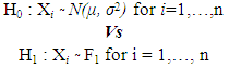 Where F1 denotes a distribution different from the normal distribution. We proceed by reviewing a few of the more common testing procedures.
2.3. Empirical Distribution Function (EDF) Tests
The idea of the EDF tests in testing normality of data is to compare the empirical distribution function which is estimated based on the data with the cumulative distribution function (CDF) of normal distribution to see if there is a good agreement between them. Dufour et al. (1998) described EDF tests as those based on a measure of discrepancy between the empirical and hypothesized distributions. The EDF tests can be further subdivided into those belong to supremum and square class of the discrepancies. Arshad et al. (2003) and Seier (2002) claimed that the most crucial and widely known EDF tests are Kolmogorov-Smirnov, Anderson-Darling and Cramer Von Mises tests.
2.4. Regression and Correlation Tests
Dufour et al. (1998) defined correlation tests as those based on the ratio of two weighted least-squares estimates of scale obtained from order statistics. The two estimates are the normally distributed weighted least squares estimates and the sample variance from other population. Some of the regression and correlation tests are Shapiro-Wilk test, Shapiro-Francia test and Ryan-Joiner test.
2.5. Moment Tests
In addition to the types of normality test categorized by Seier (2002) above, there are also other types of normality test. One of these types is called the moment tests. Moment tests are those derived from the recognition that the departure of normality may be detected based on the sample moments which are the skewness and kurtosis. The procedures for individual skewness and kurtosis tests can be found in D’Agostino and Stephens (1986). The two most widely known are the tests proposed by D’Agostino-Pearson (1973) and Jarque-Bera (1987).
2.6. Chi Square Test
The oldest and most well-known goodness-of-fit test is the CSQ test for goodness of fit, first presented by Pearson (1900). However, the CSQ test is not highly recommended for continuous distribution since it uses only the counts of observations in each cell rather than the observations themselves in computing the test statistic.
3. Simulation Result
This study employs Monte Carlo experiment to empirically investigate the power of SW, AD, CSQ, CVM, and JB test statistics to verify if a random sample x of size n independent observations come from a normal population. The random samples were generated independently in R environment. In which SW, AD, CSQ, CVM and JB were accessed via Shapiro.test, ad.test, pearson.test, cvm.test and jarque.bera.test functions respectively. Since there is no standard setting that has been established in research for empirical simulation studies for tests of normality. In the conducted studies of this work we tried to choose our parameters as conventional as possible.Seven different sample sizes n = (10, 30, 50, 100, 300, 500 & 1000) relating to small, medium, and large sample sizes were iterated over 1000 times from each of the selected alternative distributions and the levels of significance considered were 1%, 5% and 10%.The simulated samples were generated in order to test the hypotheses as follow: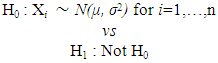 The alternative non-normal distributions were classified in accordance to Shapiro et al. (1968), which proposed the classification of continuous non-normal distributions by their skewness
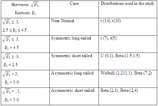
  and kurtosis (β2) into five categories, which are: Near normal distribution, Symmetric long-tailed distribution, Symmetric short-tailed distribution, Asymmetric long-tailed distribution, and Asymmetric short-tailed distribution. Then the different non-normal distributions considered in this study are essentially a subset of those investigated by Shapiro et al. (1968), Chaichatschwal & Budsaba (2007) and Yap & Sim (2010), in order to complement their results and examine whether the present study agrees or disagrees with previous ones.
 Table 1. Classification of distributions under study
 |
| |
|
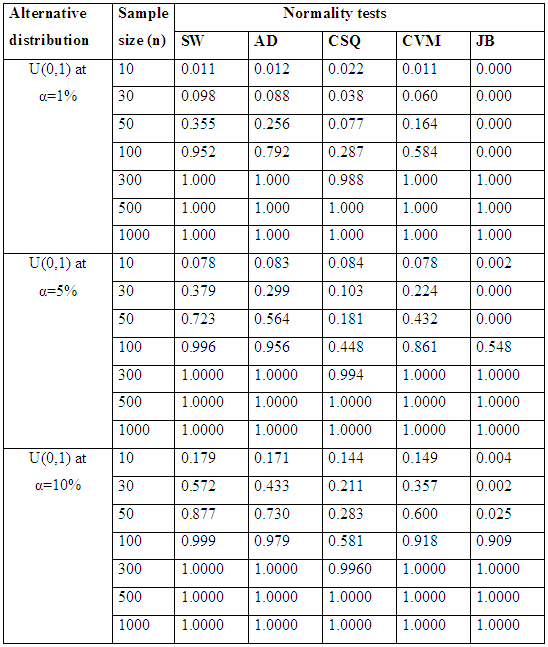
Table 2.1. Simulated Power of the near normal distributions
 |
| |
|
 | Figure 1.1. Simulated Power of the near normal distributions at various alpha levels |
Table 2.1 show the simulated power for selected Near normal distributions, while Figure 1.1 show the plot of power for all tests against selected near normal distributions for 1%, 5% and 10% significance levels. Which reveal that: for Near Normal distributions, the power of JB have better power compared to others, at all significance levels considered in the study. And the result also shows that the power of CSQ is very poor and it required much larger sample size to achieve comparable power with other tests. It can also be observed that as alpha increases, the power of the tests also increased. Table 2.2. Power for all tests against selected near normal distributions
 |
| |
|
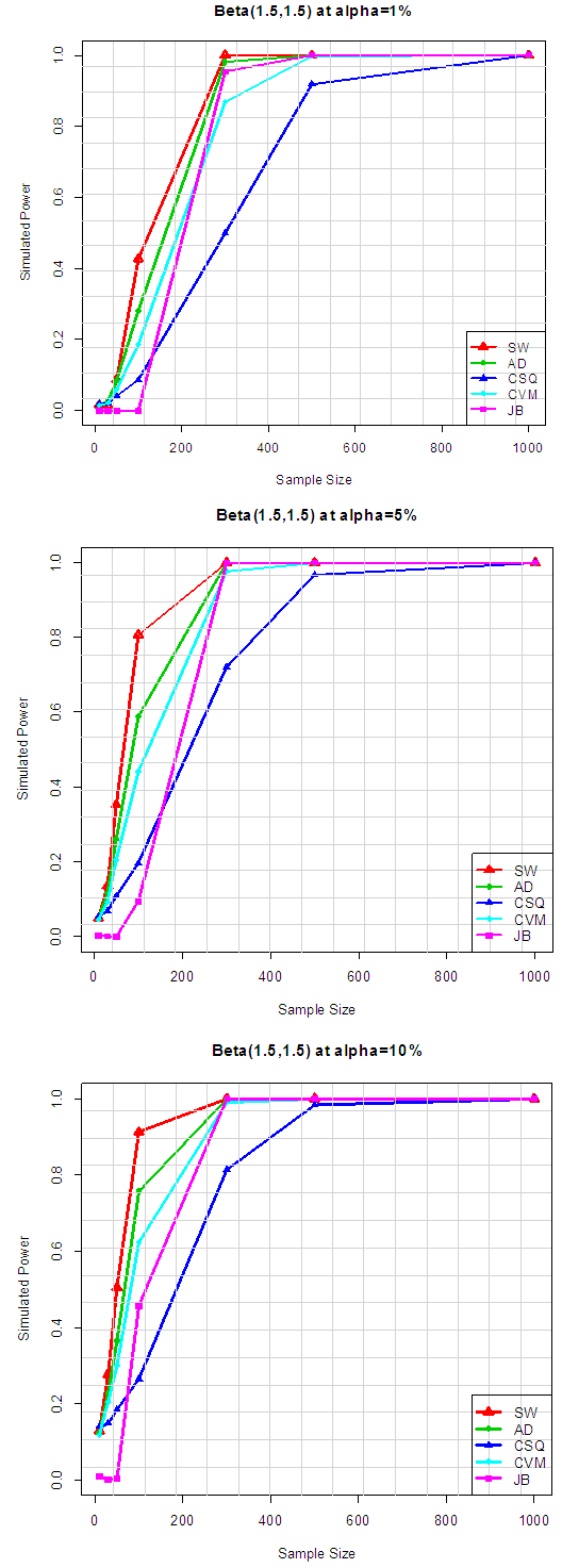
 | Figure 1.2. Power for all tests against selected near normal distributions |
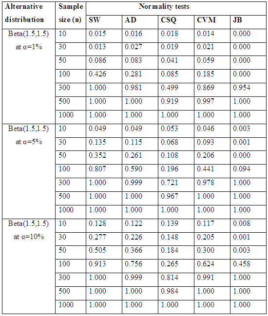
Table 2.2 and Figure 1.2 also show the plot of power for all tests against selected near normal distributions for 1%, 5% and 10% significance levels. Which reveal that: for Near Normal distributions, the power of JB have better power compared to others, follow by SW at all significance levels considered in the study. And the result also show that the power of CSQ is very poor and it required much larger sample size to achieve comparable power with other tests. It can also be observed that as alpha increases, the power of the tests also increased.Table 3.1. Simulated Power of the Symmetric long- tailed distributions
 |
| |
|
 | Figure 2.1. Power for all tests against selected Symmetric long-tailed distribution |
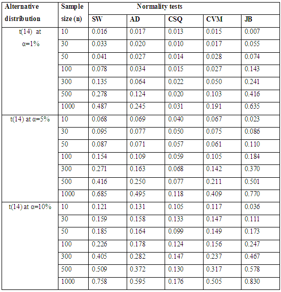
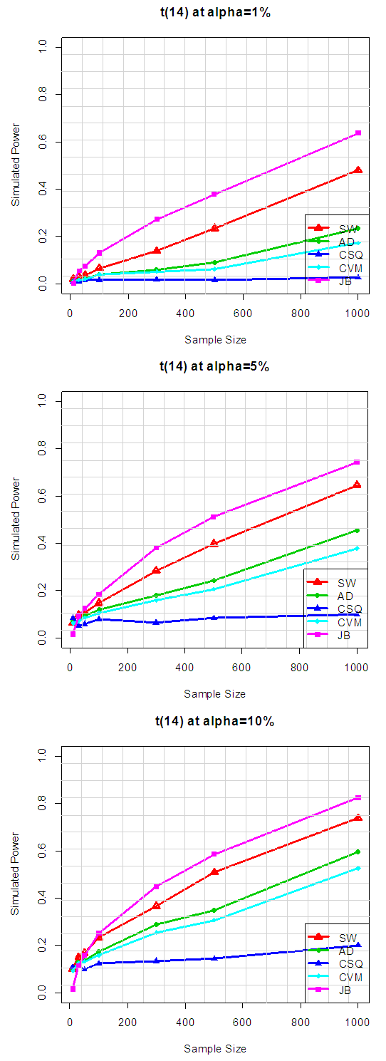
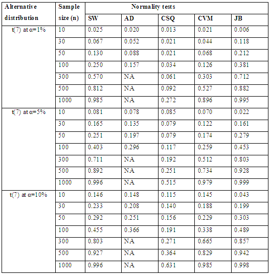
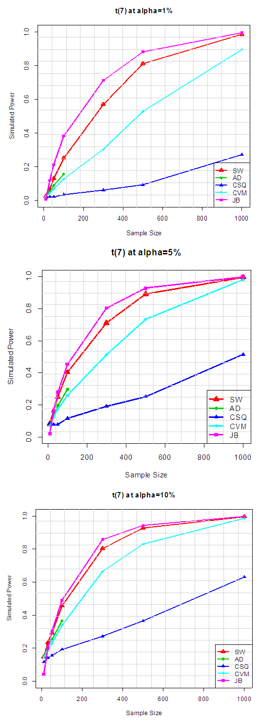
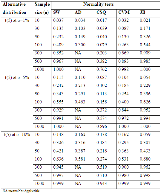
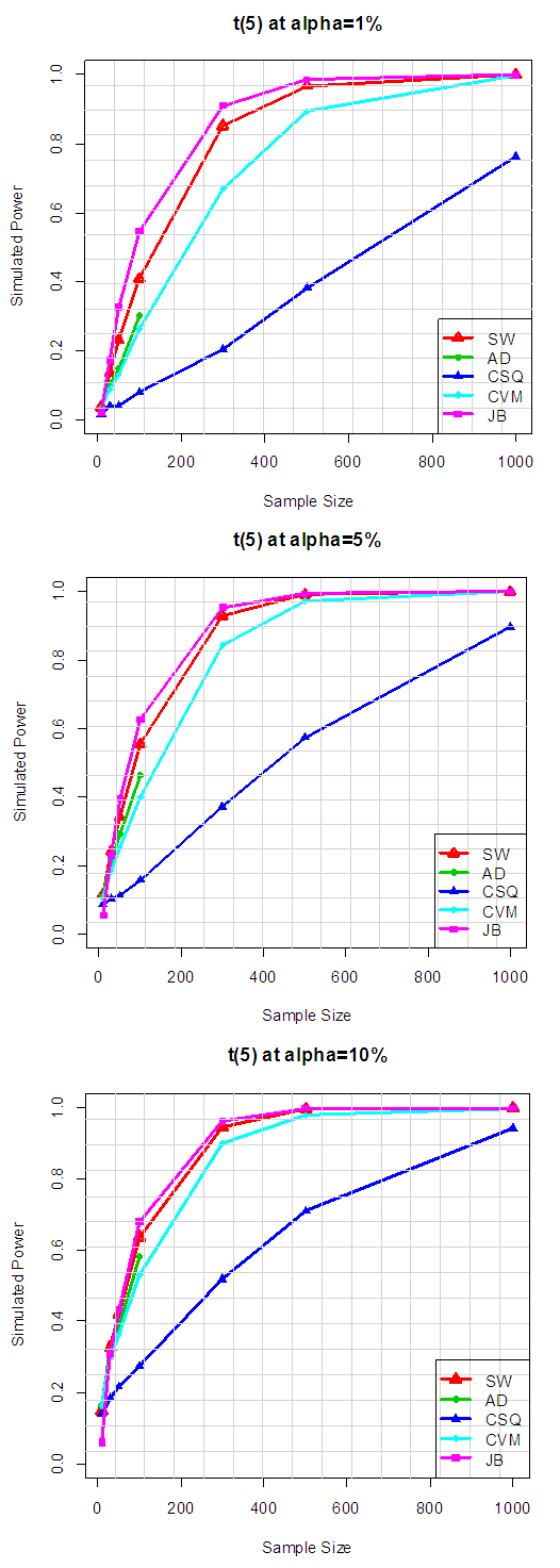
Table 3.1 shows the simulated power for selected Symmetric long-tailed distributions, while Figure 2.1 show the plot of power for all tests against selected Symmetric long-tailed distribution for 1%, 5% and 10% significance levels. Which show that: for Symmetric long-tailed distributions, the power of JB is the best, follow closely by SW at all level of significance. And also show that the power of CSQ is very low compares to other tests. Table 3.2. Power for all tests against selected Symmetric long-tailed distribution
 |
| |
|
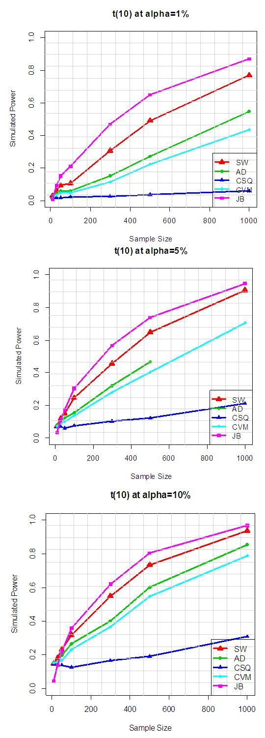
 | Figure 2.2. Power for all tests against selected Symmetric long-tailed distribution |
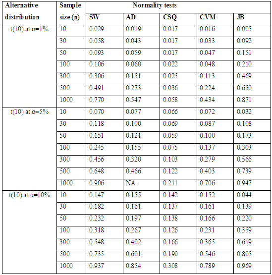
Table 3.2 shows the simulated power for selected Symmetric long-tailed distributions, while Figure 2.2 show the plot of power for all tests against selected Symmetric long-tailed distribution for 1%, 5% and 10% significance levels, which show that: for Symmetric long-tailed distributions, the power of JB is the best, follow closely by SW at all level of significance. And also show that the power of CSQ is very low compares to other tests. 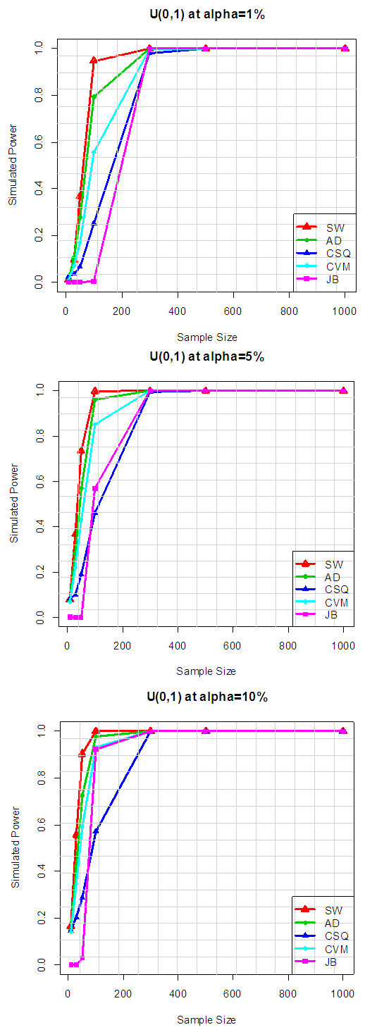 | Figure 3.1. Simulated Power of the Symmetric short tailed distributions |
Table 4.1. Simulated Power of the Symmetric short tailed distributions
 |
| |
|
Table 4.1 and Figure 3.1 reveal that, for symmetric short-tailed distributions, the power of SW is the best followed closely by AD and CVM tests and the power of JB and CSQ are relatively low, though, JB outperform CSQ. Table 4.2. Power for all tests against selected symmetric short-tailed distributions
 |
| |
|
 | Figure 3.2. Power for all tests against selected symmetric short-tailed distributions |
Table 4.2 and Figure 3.2 reveal that, for symmetric short-tailed distributions, the power of SW is the best followed closely by AD and CVM tests and the power of JB and CSQ are relatively low, though, JB outperform CSQ.Table 5.1. Simulated Power of the Asymmetric long-tailed distributions
 |
| |
|
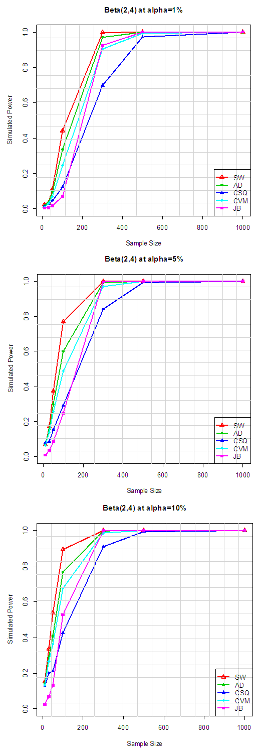
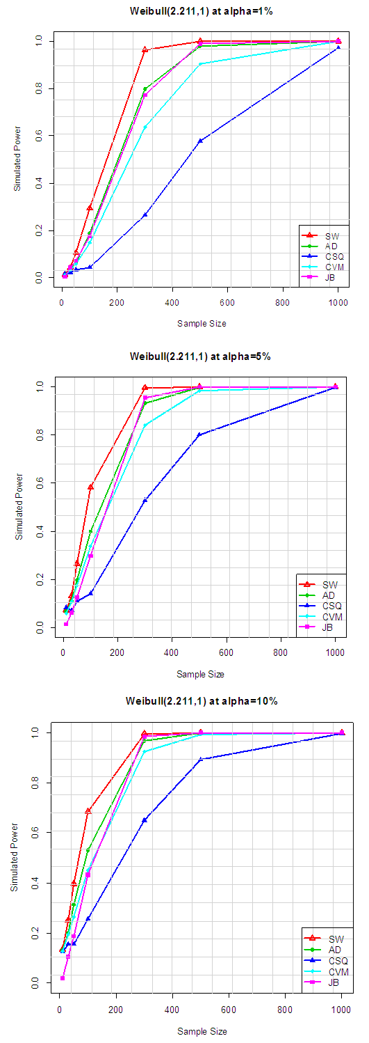 | Figure 4.1. Simulated Power of the Asymmetric long-tailed distributions |
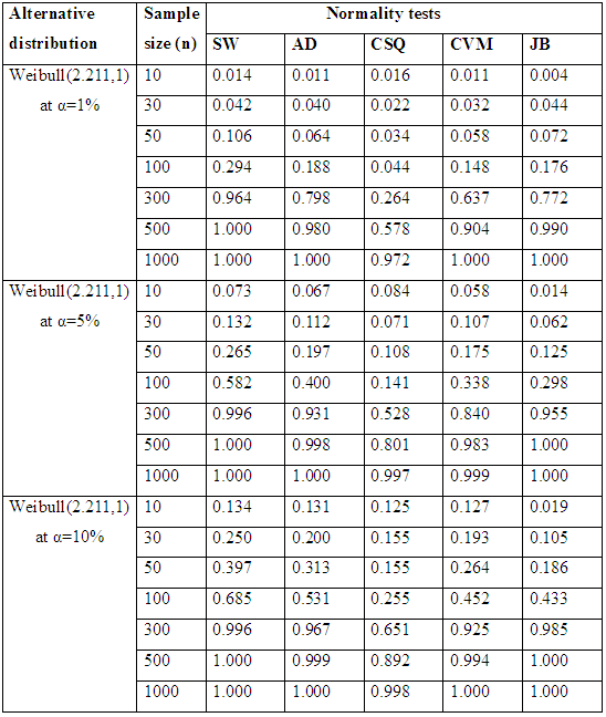
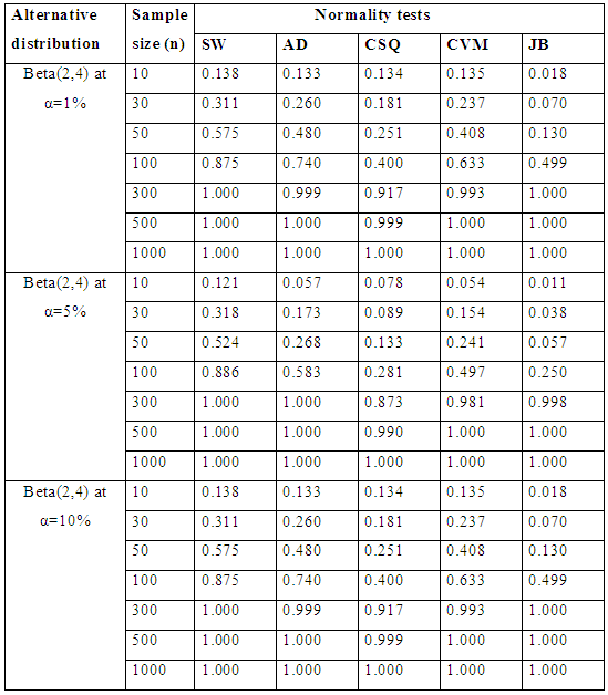
Table 5.1 summarize the simulated power for selected asymmetric long-tailed distributions for α =1%, 5% and 10%, while Figure 4.1 show the plot of power for all tests against selected asymmetric long-tailed distributions for all level of significance considered. They show that, for asymmetric long-tailed distributions, SW outperforms AD, CVM, JB and CSQ tests.Table 5.2. Simulated power for selected asymmetric long-tailed distributions
 |
| |
|
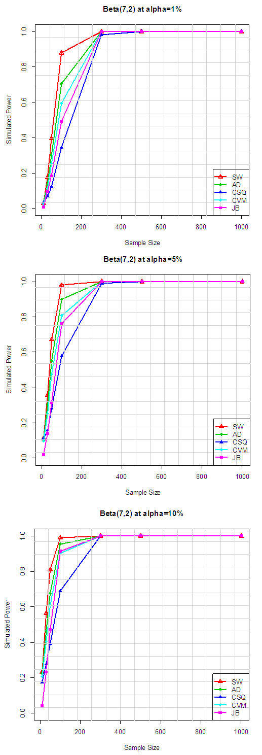 | Figure 4.2. Simulated power for selected asymmetric long-tailed distributions |
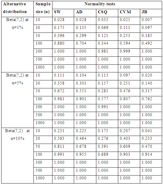
Table 5.2 summarize the simulated power for selected asymmetric long-tailed distributions for α =1%, 5% and 10%, while Figure 4.2 show the plot of power for all tests against selected asymmetric long-tailed distributions for all level of significance considered. Again for asymmetric long-tailed distributions, SW outperforms AD, CVM, JB and CSQ tests.Table 6.1. Simulated Power of the Asymmetric short-tailed distributions
 |
| |
|
 | Figure 5.1. Simulated Power of the Asymmetric short-tailed distributions |
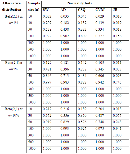
Table 6.1 reveals the simulated power for selected asymmetric short-tailed distributions for α =1%, 5% and 10% while Figure 5.1 show the plot of power for all tests against selected asymmetric long-tailed distributions for 1%, 5% and 10% significance levels. Also for asymmetric long-tailed distributions, SW outperforms other tests.Table 6.2. Simulated power for selected asymmetric short-tailed distributions
 |
| |
|
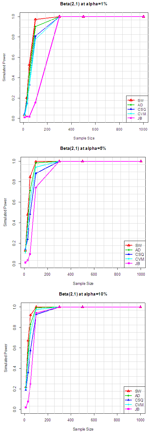 | Figure 5.2. Simulated power for selected asymmetric short-tailed distributions |
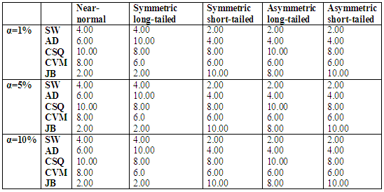
Table 6.2 reveals the simulated power for selected asymmetric short-tailed distributions for α =1%, 5% and 10% while Figure 5.2 show the plot of power for all tests against selected asymmetric long-tailed distributions for 1%, 5% and 10% significance levels. Also for asymmetric long-tailed distributions, SW outperforms other tests.In order to get a clear picture of the performance of these normality test. The ranking procedure was employed. The rank of 1 was given to the test with the highest power while rank of 5 was given to the test which has the lowest power (since there were five tests of normality considered in this study). The ranks were then summed to get the grand total of ranks. As the lowest number was given to the test with the highest power, therefore the test which had the lowest total rank was nominated as the best test to detect the departure from normality. Table 7.1 and Table 7.2 show the rank of power based on sample size and the type of alternative distribution, respectively.The results of the total rank based on sample size in Table 7.1 below show that SW has the best test for all sample size since it consistently has the lowest total rank for all sample sizes considered. Also from Table 7.2, it can be clearly seen that JB is the best test to be adopted for Near normal and Symmetric long-tailed distributions, and it is followed closely by SW. While SW is the best test to be adopted for both symmetric short-tailed, asymmetric long-tailed and asymmetric short-tailed distribution, and it is followed rather closely by the AD test since it has the lowest total rank (for all level of significances) among all the five tests considered. Table 7.1. Rank of power based on sample size for all the alternative distributions
 |
| |
|
Table 7.2. Rank of power based on the type of Alternative distribution
 |
| |
|
4. Conclusions
In general, it can be concluded that:I. The powers of all the tests considered in this study increases as the sample size and significance level increases. This is in agreement with the findings of Razali et al. (2010). II. The results also supports the finding of Oztuna et. al. (2006) that the SW test has good power properties over a wide range of non-normal distributions.III. In consonance with the finding of Nakagawa et al. (2007), the JB power is very poor for Symmetric short-tailed distribution. But if the distribution is near normal and symmetric long-tailed, then JB tests is considered to be appropriate. IV. The results also agree with Stephen (1993) who reported that CSQ tests for normality have poor power property for all the alternative continuous non-normal distribution.Finally, based on the findings from this study and in concurrence with relevant literature reviewed, it was discovered that most of these normality tests were developed in the 1960s, 1970s and 1980s. After the development of the Jarque-Bera test in the late 1980s, only few new tests seemed to appear after that time. However, none of these new tests could establish itself as a real alternative for testing normality with an essential improvement of empirical power behavior. This leads us to the conclusion that the theory of testing for normality, in particular the search for the tests of normality with better power behavior than the already existing tests seems to be mostly closed.
5. Recommendations
As a concluding remark, it is recommended that a researcher should combine the graphical technique with formal normality test and also some measures of skewness and kurtosis should be put in consideration before choosing the appropriate normality test in order to avoid erroneous conclusion.
References
| [1] | Anderson, T.W., and Darling, D.A., A Test of Goodness of fit, Journal of the American Statistical Association, 49; 1954: 765-769. |
| [2] | Shapiro, S.S., and Wilk, M.B., An Analysis of Variance Test for Normality, Biometrika, 52; 1965: 591-611. |
| [3] | Shapiro, S.S., Wilk, M.B. and Chen, H.J., A Comparative Study of Various Tests for Normality, Journal of the American Statistical Association, 3; 1968: 343-1370. |
| [4] | Tae-Hwan Kim and Halbert White, On More Robust Estimation of skewness and Kurtosis: Simulation and Application to the S&P500 Index. |
| [5] | Thomas A. Ryan, Jr. and Brian L. Joiner, Normal Probability Plots and Tests for Normality, Statistics Department, The Pennsylvania State University 1976. |
| [6] | Derya Öztuna, Elhan, and Tüccar, Investigation of Four Different Normality Tests in Termsof Type 1 Error Rate and Power under Different Distributions, Turk J Med Sci, 2006; 36 (3): 171-176. |
| [7] | Seier Edith, Douglas G. Bonett, A test of Normality with high uniform power, Computational statistics & Data Analysis 40 (2002) 435-445. |
| [8] | Nakagawa, Niki and Hashiguchi. An Omnibus test for normality. Proc. of the ninth Japan-China sympo. On Statistics. 191-194, 2007. |
| [9] | M.A. Stephens. EDF Statistics for Goodness of fit and some comparison. Journal of the American statistical Assocition. Vol. 69, No. 347 (sept, 1974), 730-737. |
| [10] | Nornadian Mohd Razali, Yap Bee Wah. Power comparisons of some selected normality tests. Proceedings of the Regional Conference on Statistical Sciences 2010 (RCSS’10) June 2010, 126-138. |
| [11] | James Brown D. Shiken: JALT Testing & Evaluation SIG Newsletter, 1 (1) April 1997 (p. 20-23). |
| [12] | R. C. Geary. Testing for Normality. Biometrika, Vol. 34, No. 3/4. (Dec., 1947), pp. 209-242. |
| [13] | M.A Stephen, Aspect of Goodness of fit, Technical report No. 474. Sept. 30, 1993. |
| [14] | Oja, H., 1981. On location, scale, skewness and kurtosis of univariate distributions. Scand. J. Statist. 8, 154–168. |
| [15] | Jean-Marie Dufour, Abdeljelil Farhat, Lucien Gardio, Lynda Khalaf. Simulation-based finite sample normality tests in linear regressions. Econometrics Journal (1998), volume 1, pp. 154-173. |
| [16] | Hun Myoung Park, 2008. Hypothesis Testing and Statistical Power of a Test. Working Paper. The University Information Technology Services (UITS) Center for Statistical and Mathematical Computing, Indiana University.” http://www.indiana.edu/~statmath/stat/all/power/index.html. |

 Abstract
 Reference
 Full-Text PDF
 Full-text HTML