1. Introduction

Count data is a statistical data type, a type of data in which the observations can take only the non-negative integer values {0, 1, 2, 3, ...}, and where these integers arise from counting rather than ranking [1-3]. The statistical treatment of count data is distinct from that of binary data, in which the observations can take only two values, usually represented by 0 and 1, and from ordinal data, which may also consist of integers but where the individual values fall on an arbitrary scale and only the relative ranking is important. Count data models have a dependent variable that is counts (0, 1, 2, 3, and so on) [4]. Most of the data are concentrated on a few small discrete values. Examples include: the number of children a couple has, the number of doctor’s visit per year a person makes, and the number of trips per month that a person takes. Count data arise in many fields which includes; biology, healthcare, psychology, marketing and many more. When response variable is a count and the researcher is interested in how this count changes as the explanatory variable increases. Classical Poisson regression is the most well-known methods for modeling count data, but its underlying assumption of equidispersion limits its use in many real-world applications with over-or under dispersed data [5-7]. This excess variation may result to incorrect inference about parameter estimates, standard errors, tests and confidence intervals. Over-dispersion mostly arises for various reasons including mechanisms that generate excessive zero counts or censoring [9-11]. As a result over-dispersed count data are common in many areas which in turn, have led to the development of statistical methodology for modeling over-dispersed data. For over-dispersed data, the Negative Binomial model is a popular choice. Other over-dispersion models include Poisson mixtures and Conway-Maxwell-Poisson. A flexible alternative that captures both over- and under-dispersion is the Conway-Maxwell-Poisson (COM-Poisson) distribution. The COM-Poisson is a two-parameter generalization of the Poisson distribution which also includes the Bernoulli and Geometric distributions as special cases [12]. The COM-Poisson distribution has been used in so many count data application and has been extended methodologically in various directions. Therefore in this work, because of the problem of model selection and the appropriate method to apply in the analysis of auto-crash data bearing in mind their underlying assumptions, we wish to find the model that is most adequate.

2. Materials and Method

In this section we shall review the models that most widely used in the analysis of count data which include: the Poisson models, Conway- Maxwell- Poisson models, Generalized Poisson Regression model, and the Negative Binomial Regression Model.

2.1. Poisson Models

This is a special case of Generalized Linear Models (GLM) framework. The simplest distribution used for modeling count data is the Poisson distribution with probability density function.

For . The mean and variance of this distribution can be shown to be . Since the mean is equal to the variance, any factor that affects one will also affect the other. Thus, the usual assumption of homoscedasticity would not be appropriate for Poisson data.

Suppose that we have a sample of n observations which can be treated as realizations of independent Poisson random variables, with and suppose that we want to let the mean µ_i (and therefore the variance) depend on a vector of explanatory variables [13-15].

We could entertain a simple linear model of the form

but this model has the disadvantage that the linear predictor on the right hand side can assume any real value, whereas the Poisson mean on the left hand side, which represents an expected count, has to be non-negative. A straightforward solution to this problem is to model instead the logarithm of the mean using a linear model. Thus, we take logs calculating

and assume that the transformed mean follows a linear model

Thus, we consider a generalized linear model with link log. Combining these two steps in one we can write the log-linear model as

In this model the regression coefficient represents the expected change in the log of the mean per unit change in the predictor . In other words increasing by one unit is associated with an increase of in the log of the mean. Exponentiating the above equation, we obtain a multiplicative model for the mean itself:

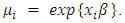In this model, an exponentiated regression coefficient represents a multiplicative effect of the predictor on the mean. Increasing by one unit multiplies the mean by a factor . A further advantage of using the log link stems from the empirical observation that with count data the effects of predictors are often multiplicative rather than additive [16]. That is, one typically observes small effects for small counts, and large effects for large counts. If the effect is in fact proportional to the count, working in the log scale leads to a much simpler model.

The Likelihood function for the Poisson model is;

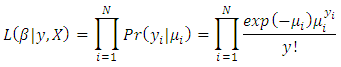
2.2. Conway-Maxwell-Poisson (COM-Poisson) Models

The Conway Maxwell Poisson (COM-Poisson) distribution with two parameters was originally developed as a solution to handling queueing systems with state-dependent arrival or service rates. This distribution generalizes the Poisson distribution by adding a parameter to model over-dispersion and under-dispersion and includes the geometric distribution as a special case and the Bernoulli distribution as a limiting case. The COM-Poisson distribution is a two parameter generalization of the Poisson distribution that is flexible enough to describe a wide range of counts data distributions, since its revival, it has been further developed in several directions and applied in multiple fields.

The COM-Poisson probability distribution function is given by the equation:

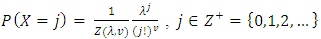Where is a normalizing constant defined by

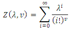The domain of admissible parameters for which defines a probability distribution is . The introduction of the second parameter ν allows for either sub or super-linear growth of the ratio , and allows X to have variance either less than or greater than it’s mean. Of course, the mean of is not, in general, λ. Clearly, in the case where 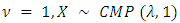has the Poisson distribution and the normalizing constant 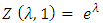. Note, other choices of ν also give rise to well-known distributions. For example, in the case where and , X has a geometric distribution, with 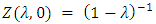. In the limit , X converges in distribution to a Bernoulli random variable with mean and lim 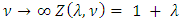. In general, of course, the normalizing constant does not permit such a neat, closed-form expression. Asymptotic results are available, however. Gillispie and Green [17] prove that, for fixed ν,

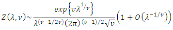As , confirming a conjecture made by Shmueli et al [18-19]. This asymptotic result may also be used to obtain asymptotic results for the probability generating function of , since it may be easily seen that

2.3. The Generalized Poisson Regression Model

The advantage of using the generalized Poisson regression model is that it can be fitted for both over-dispersion, , as well as under-dispersion, . Suppose is a count response variable that follows a generalized Poisson distribution, the probability density function of is given as (Famoye (1993), Wang and Famoye (1997)) [20];

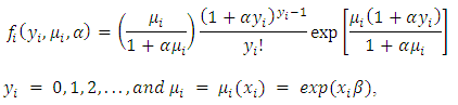Where is a dimensional vector of covariates including demographic factors, driving habits and medication use, and is a dimensional vector of regression parameters. For details on the generalized Poisson regression model, the reader is referred to Famoye (1993) [21]. The mean and variance of are, respectively, given by

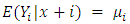and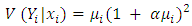

The generalized Poisson regression model above is a generalization of the standard Poisson regression (PR) model. When the probability function model, the equality constraint is observed between the conditional mean and the conditional variance of the dependent variable for each observation. In practical applications and in “real” situations, this assumption is questionable since the variance can either be larger or smaller than the mean. If the variance is not equal to the mean, the estimates in PR model are still consistent but are inefficient, which leads to the invalidation of inference based on the estimated standard errors.

2.4. Negative Binomial Regression

Negative binomial regression is similar to regular multiple regression except that the dependent (Y) variable is an observed count that follows the negative binomial distribution. Thus, the possible values of Y are the nonnegative integers: 0, 1, 2, 3, and so on. Negative binomial regression is a generalization of Poisson regression which loosens the restrictive assumption that the variance is equal to the mean made by the Poisson model. The traditional negative binomial regression model, commonly known as NB2, is based on the Poisson-gamma mixture distribution. This formulation is popular because it allows the modelling of Poisson heterogeneity using a gamma distribution [22].

The Poisson distribution may be generalized by including a gamma noise variable which has a mean of 1 and a scale parameter of ν. The Poisson-gamma mixture (negative binomial) distribution that results is

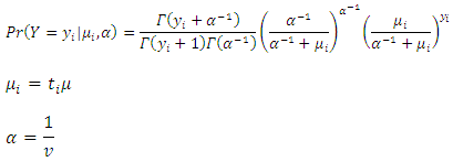The parameter is the mean incidence rate of y per unit of exposure. Exposure may be time, space, distance, area, volume, or population size. Because exposure is often a period of time, we use the symbol to represent the exposure for a particular observation. When no exposure given, it is assumed to be one. The parameter may be interpreted as the risk of a new occurrence of the event during a specified exposure period, t.

The results below make use of the following relationship derived from the definition of the gamma function

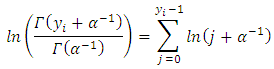In negative binomial regression, the mean of y is determined by the exposure time t and a set of k regressors variables (the x’s). The expression relating these quantities is

Often, , in which case is called the intercept. The regression coefficients are unknown parameters that are estimated from a set of data. Their estimates are symbolized as . Using this notation, the fundamental negative binomial regression model for an observation i is written as

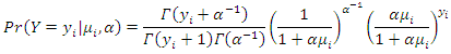
2.5. Multicollinearity Test

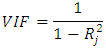
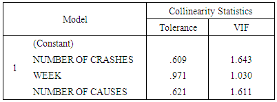
One formal way of detecting Multicollinearity is by the use of the variance inflation factors (VIF) [23]. The VIF is used to test for the presence of Multicollinearity, and is given by

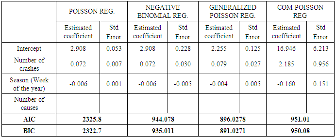
Where is the coefficient of determination of a regression of an explanatory variable j on all the other explanatory variables. A VIF value of 10 and above indicates a Multicollinearity problem.

Table 1 shows that all the variables have VIF values <10. Thus all the variables can be included in the subsequent analyses and modeling with the Poisson regression, Generalized Poisson regression, and Negative Binomial Regression.

Table 1. Multicollinearity Test

2.6. Akaike Information Criterion (AIC)

When several models are available, one can compare the models performance based on several likelihood measures which have been proposed in statistical literatures. One of the most popularly used measures is AIC [24-25]. The AIC penalized a model with larger number of parameters, and is defined as

Where denotes the fitted log likelihood and 𝑝 the number of parameters. A relatively small value of AIC is favorable for the fitted model.

2.7. Bayesian Information Criterion (BIC)

The Bayesian information criterion (BIC) or Schwarz criterion (also SBC, SBIC) is a criterion for model selection among a finite set of models; the model with the lowest BIC is preferred [26]. It is based, in part, on the likelihood function and it is closely related to the Akaike information criterion (AIC).

When fitting models, it is possible to increase the likelihood by adding parameters, but doing so may result in overfitting. Both BIC and AIC attempt to resolve this problem by introducing a penalty term for the number of parameters in the model; the penalty term is larger in BIC than in AIC.

The BIC is formally defined as

Where,

the maximized value of the likelihood function of the model.

n = the number of data points in the observed data, the number of observations, or equivalently, the sample size.

k = the number of parameters estimated by the model.

3. Results and Discussion

Auto crash data was collected from the Federal Road Safety Corps National Headquarters Abuja and data wase analyzed using R Software and the results obtained are given below. Before performing the analysis on the four methods used, the data were tested for Multicollinearity. The test results are shown on the table below.

Table 2. Parameter estimates, standard error and AIC value for the models

4. Conclusions and Recommendations

Poisson Regression Model, Generalized Poisson Regression Model, Negative Binomial Regression Model, and Conway-Maxwell Poisson regression model were compared to determine a better model used in modeling auto-crashes in Nigeria. The criterion for selection of the best model used is AIC and BIC values. Best model is the model that has the smallest AIC and BIC value.

Based on the values on Table 2 above, the model with the smallest AIC and BIC value is the Generalized Poisson Regression model. Thus, the best model for analyzing traffic crash data in Nigeria is the Generalized Poisson Regression model.