1. Introduction

In financial econometrics, managing risks associated with volatility is a key function of the currency market in the current worldwide. Due to uncertainties, in the factors of the money markets, specialists of the finance and the econometrics are dealing with the time series modeling to analyze the behavior of the currency volatility. GARCH family models are now being considered as the most prominent tools for capturing the changes. It is assumed that series are distributed normally with mean zero and constant variance which is varies over the time [1]. The aim of this study is to reflect symmetric and asymmetric response patterns of GARCH family models using volatility effect.

As the initial step, Black (1976) and Christie (1982) were investigated the relationship between returns and volatility, concluding with negative relationship for the asymmetric effect [2]. Engle, R. F. (1982) and Bollerslev (1986) introduced the symmetric effects of time series modeling. ARCH(p) was introduced by Engle (1982). ARCH model can be used to model the effects of serial correlation and the conditional heteroskedasticity. Later in 1986 Bollerslev found the solution for the drawbacks of ARCH model as the GARCH(p,q) model. In GARCH model the conditional variance expressed as a function of constant, volatility terms and variance terms.

In order to capture asymmetry Nelson (1991) proposed exponential GARCH process or EGARCH for the conditional variance: the GJR-GARCH model introduced by Glosten, Jagannathan and Runkle (1993). Therefore while the GARCH model imposes the nonnegative constraints on the parameters, EGARCH models the log of the conditional variance so that there are no restrictions on these parameters [3]. This is an extension GARCH where the indicator function or the dummy variable, equals 1 if the residue of the previous period is negative and zero otherwise. Ding, Granger and Engle (1993) proposed a model that extends the class of GARCH specifications to analyze a broader class of transformations taking account of the power effect. Zakoian (1994) proposed TGARCH (p,q) model as alternative to EGARCH process, where asymmetry of positive and negative innovations is incorporated in the model by using indicator function: Models with threshold effect are piecewise linear models that describe the variability of the conditional deviation and not the conditional variance as all other GARCH specifications.

This Study attempts to compare the symmetric and asymmetric effects of GARCH models, with the usage of volatility of exchange rate in Sri Lanka against five currencies which are related to the top level economy in the world context.

2. Literature Review

2.1. Symmetric and Asymmetric Effects of GARCH Models on ERV

The study by Narsoo [4], on modeling and forecasting exchange rate volatility using daily data, over the period of six years revealed the predictive ability of symmetric models compared to the asymmetric models focusing on GARCH family, concluding the suitability of asymmetric models in predicting the USD/MUR exchange rate volatility. According to Kutu and Ngalawa [5], exchange rate of South Africa is significantly affected by global shocks by employing symmetric GARCH(p,q) model. Omari et al [6] investigated the volatility clustering and leverage effects, concluding that daily exchange rate returns are characterized by GARCH family models such as symmetric GARCH(1,1) and GARCH-M(1,1) and asymmetric EGARCH, TGARCH & APARCH in (1,1) level. Abdalla [7] defined the same using GARCH and EGARCH for nineteen Arab countries.

Research by Epaphra [8], suggested that behavior of exchange rates are effected by the prior data related to the exchange rates, additionally asymmetric volatility suggest positive shocks than negative shocks resulting the exchange rate volatility and transaction cost are correlated positively, thus profits to international trade negatively correlated. Bala and Asemota [9] remarked that most of the asymmetric models except the models with volatility breaks refuse the leverage effects. David, O.R. Dikko, H.G. and Gulumbe, S.U. [10] highlighted Naira exchange rate volatility using GARCH (1,1) and its asymmetric variants. The results indicated selected determinants are significant and different impacts of both positive and negative shocks. Ntawihebasenga et al. [11] defined, some drawbacks of difficulty of measuring persistence and lack of symmetry in response to shocks using GARCH models. Rwandese foreign exchange market data was used for the analysis, for the period of June 2009 to June 2014. GARCH, EGARCH and TGARCH models were used by Vojcic [12] for the evaluation of volatility performance. Results indicate that compared to the Gaussian distribution, Student t distribution fits the data. Thus positive shocks are less influenced on volatility compared to the negative shocks.

2.2. Exchange Rate Volatility on Economic Growth

Sandoval [13] focus on the asymmetric GARCH models, for the better fit of exchange rate volatilities, concluding two assumptions. First analyst must be aware about the possible effects of asymmetry. Secondly, analyzing in-sample data will obtain the optimum result than the out-of-sample data for the emerging exchange rate series. Clerk, et al. [14] examined the exchange rate volatility on trade, using a panel data set, covering 178 countries. The results reveal, some developments show exacerbated fluctuations, thus others reduce the impact on exchange rate volatility in the world market. According to Kohler et al. [15], pointed out the effects of exchange rate movements in economic activity and inflation in Australia. He suggested over one to two years less than half per cent of level of GDP can be increased by decreasing the exchange rates by ten percent temporary. Further domestic industries are influenced less than the trading industries. Minh et al. [16] investigated the impact of exchange rate volatility and FDI on agricultural sector. It is concluded with fluctuations in exchange rate volatility affects negatively on agricultural production while FDI is insignificant on the agricultural production. Zamir et al. [17] focused on the effects of exchange rate volatility on foreign exchange reserves and some other variables. The study highlighted that exchange rate volatility is influenced negatively on foreign exchange reserves. Increasing exports needs the devaluation of rupee values, thus better to follow import substitution policies. Wang et al. [18] remarked the estimation of exchange rate risk and keep the optimal portfolio of foreign exchange using RMB exchange rates against dollar and yen for year 2008-2012 using Copula-GARCH model. Rofael and Hosni [19] pointed out the dynamics of the exchange rate modeling using ARCH family models, concluded with Egypt is suffering from volatility clustering, thus exists a time-varying variance in the series of exchange rates. There is a risk mismatch between the volatility of exchange market and the stock market.

3. Methodology

3.1. Symmetric Effects of GARCH Models

Consider Y_t is a stationary time series,

Where σ_t ≥ 0, it is generated by Y_t-k , k ≥ 1 and ε_t denotes the variable which is randomly distributed and independent with mean zero and variance equals to one defined by a volatility model.

Modeling exchange rate return series, ARCH is defined as the value added model under the temporal dependencies. It is a function of past squared returns which was proposed by Engle (1982) as a very first series with the effects if heteroscedasticity and volatility clustering. ARCH(q) model can be illustrated as:

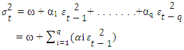Where,

ω > 0, α_i ≥ 0 for i=1,2,3,….,q and

If the 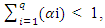then it is considered as the return process is weekly stationary, then the unconditional variance can be defines as:

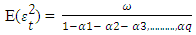ARCH(1) can be derived from ARCH(q) model, if denote as the Conditional Variance of Random Variable, then ARCH(1) can be showed as,

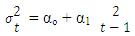Bollerslev (1986) introduced the Generalized ARCH model as an extension of ARCH(q) model. The GARCH model can be typically defined as:

Where Y_t denotes the exchange rate returns and µ as mean value, µ ≥ 0:

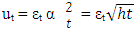Where ε_t ~ N(0,1)

Conditional variance equation of GARCH(p,q) can be defined as:

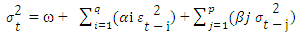Where,

Value of mean, ω > 0

α_i ≥ 0 for i=1,2,3,….,q and β_j ≥ 0 for i=1,2,3,….,p, therefore

Condition for the stationary can be derived as:

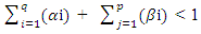Where the summation of ARCH and GARCH terms, ARCH term as the lag of squared residuals and GARCH term as the variance forecast of previous period. It is expected to be β > α.

The Generalized ARCH model is further defined by:

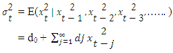Where, constant d_i ≥ 0

The GARCH(1, 1) is derived from GARCH(p,q), which the term(1,1) defined as first order autoregressive GARCH term and first order moving ARCH term. Then the model is specified as follows:

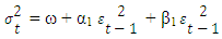Where,

ω > 0, α₁ > 0, β₁ ≥ 0 and α₁ + β₁ < 1

E(ε_t-1 | Ω) = 0

If denotes as h_t , then

Mean equation, Yt = µ + ε_t , ε_t | I_t-1 ~ N(0, h_t)

Conditional variance equation,

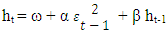Where the terms can be defined as, forecast variance, Yt , ε_t – residual term, N- conditional normal density with mean zero variance h_t , ω – mean, conditional variances as h_t-1 and the news from the previous period, Then previous period observed volatility is α and the β denotes the previous period forecast variance.

3.2. Asymmetric Effects of GARCH Models

Nelson (1991) introduced the EGARCH model for a solution of drawbacks aroused from ARCH and GARCH models which are non-negativity constraints and leverage effects. Leverage effect is an asymmetric volatility characteristic. Conditional Variance can be expressed as,

Where,

asymmetry parameter. Therefore, when there is a asymmetry effect, while indicates the volatility increases more after bad news, than after good news, denotes the conditional variance. Taking the logarithm of conditional variance ensures the non-negativity constraint, where the leverage effect is exponential in EGARCH model, Y < 0. For the symmetric affect Y≠0. This model automatically allows the lagged error to be asymmetric. Then there are no equal negative residuals for the regression residuals. captures the asymmetric response. To accept the hypothesis of no significant difference in the good or bad effects should be take zero value. That means there is no asymmetric effect. is measured the good or bad effect of the conditional variance. This was further investigated by Black (1976) [20]. Bad news is influenced more than the good news in the future volatility.

Glosten, Jagannathan and Runkle proposed the threshold GARCH(TGARCH) for symmetric effects of good news or bad news. The TGARCH model can be expressed as:

Where,

ε_t-1 < 0 denotes the good news, the total effects are (α_i + γ_i) and ε_t-1 > 0 denotes the bad news, then total effects are Negative news of exchange rate volatility identifies more fluctuations in the currency market in the global economy. If bad news influenced more than good news on the volatility, TGARCH is expected to be positive.

Ding, Granger and Engle in year 1993 proposed, one of the extensions of GARCH model with integrating the power effect, which is called the Power GARCH model (PGARCH). The PARCH specification is expressed by equation:

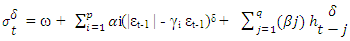Where,

X ω > 0, α_i ≥ 0 with at least one α_i > 0, i = 1,2,3,….,q and β_j ≥ 0, j = 1,2,3,…,p

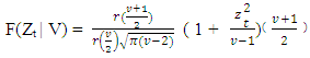
3.3. Student t Distribution

Comparison of symmetric and asymmetric GARCH effects on exchange rate volatility, it was decided to utilize the student t distribution method. This can be specified as the equation given below.

3.4. Data Description

The data consist of daily observations of exchange rates from the period of January 2010 to August 2018. The data series were obtained from the FRED database online. Daily returns are computed as the logarithm transformation of data series using the formula below:

The data sample consists of 2153 observations. 500 observations were selected as the in-sample for forecast estimation from January 2016 to August 2018.

4. Estimation Results

4.1. Graphical Representations

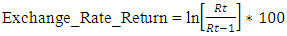
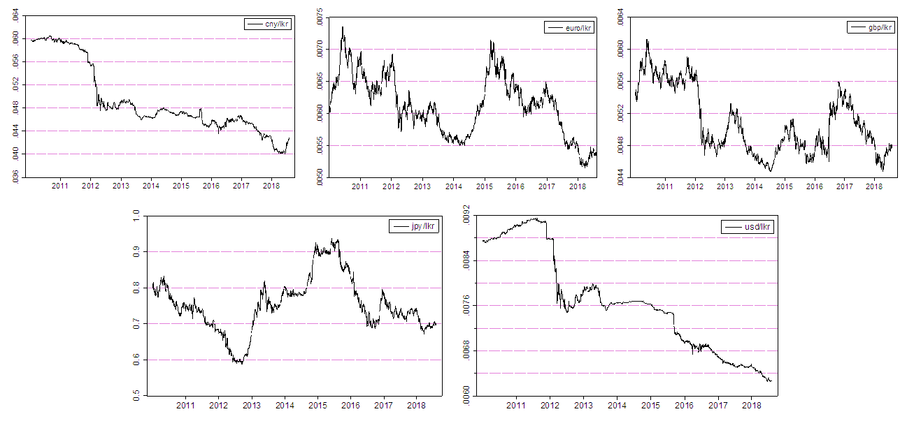
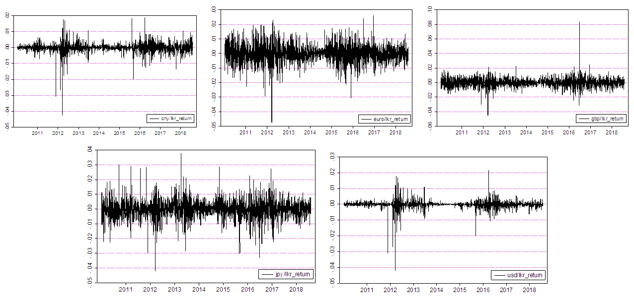
Figure 1, plots daily exchange rates in January 2010 to August 2018 period of 8 years, for a total number of 2153 observations. Top 5 economies were selected, countries as China, United Kingdom, Germany, Japan and United States for the currencies of Chinese Yuan, Sterling Pound, Euro, Japan Yen and U.S.Dollars against Sri Lankan rupees.

There is stochastic upward trend in non-stationary daily exchange rate data series over the sample period.

Figure 2 plots the changes in the daily exchange rate returns. Log difference of daily exchange rates was taken as the daily exchange rate return.

Figure 3, the Quantile-Quantile (Q-Q) plot for the exchange rates against Sri Lankan rupees.

Figure 1. Trend in Daily Exchange Rates

Figure 2. Trend in Daily Exchange Rate Returns

Figure 3. Q-Q plot of Exchange Rate Returns

4.2. Descriptive Statistics

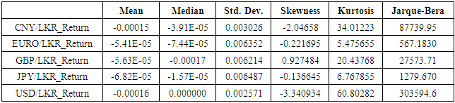
Table 1 shows the descriptive statistics of the each exchange rate return series. GBR/LKR indicates the high kurtosis and positive skewness, while other variables are negatively skewed with high kurtosis. Euro/LKR and JPY/LKR highlight the relatively low kurtosis than other series. J-B statics of return series are being indicated extremely high values. Concluding that residuals of all the exchange rate return series are not significantly normally distributed.

Table 1. Useful Statistical Indicators of Exchange Rate Returns

Table 2. Critical Values of ADF/PP Tests

4.3. Serial Correlation and Unit Root Test

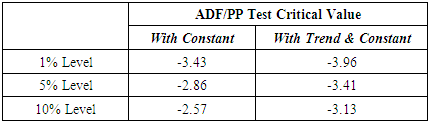
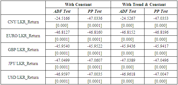
The Augmented Dickey-Fuller (ADF) and Phillip-Perron (PP) methods are conducted to check for the unit root for the Exchange Rate series in both levels and first differences. Table 3 shows the results of unit root test for daily exchange rate return series. The Augmented Dickey-Fuller test and Phillips-Perron test statistics for all exchange rate series are not significant, while significant effect of exchange rate return series means the values are less than their critical values at 1%, 5% and 10% level, thereby suggesting the rejection of null hypothesis of the absence of unit root in the original series.

Table 3. ADF and PP unit root tests of Exchange Rate Returns

4.4. Estimation of Variance Equation

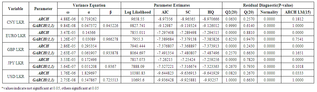
Table 4 shows variance equation estimates for the symmetric effects of exchange rate return series. Table 5 shows variance equation estimates for the Asymmetric effects of exchange rate return series. Normal (Gaussian) Distribution was selected as the method of analysis.

Table 4. Symmetric GARCH models for Exchange rate return series

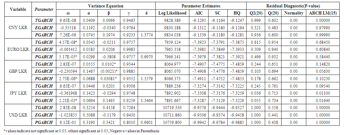Table 5. Asymmetric GARCH models for Exchange rate return series

As Table 4 indicated that, all the model parameters are significant for symmetric GARCH models in all the series. Empirical evidences stated that the sum of ARCH and GARCH coefficients lead to persistent of volatility shocks. Except USD/LKR return series other distributions indicates the sum of α and β, nearly value of one. In contrast with ARCH LM test statistics, as the p-value higher than 0.05 means that GARCH(1,1) model shows the acceptance of the null hypothesis of no serial correlation among residuals. ARCH(1) indicates the significant effect means model not suitable for volatility of exchange rates. Q-statistics are further confirming the insignificant effects of the distribution. Comparing two series, higher log likelihood with lower information criteria indicate the best fitted model for forecasting the volatility. Each of the return series are highlighted the GARCH(1,1) is the most suitable symmetric model for the volatility forecasting under the normal distribution methodology.

For the purpose of capturing asymmetry dynamics, TGARCH(1,1), EGARCH(1,1) and PGARCH(1,1) were selected as the asymmetric non-linear models for the volatility estimates under normal distribution. CNY/LKR, and USD/LKR are representing the significant effects of all the parameter estimates, while other series are having insignificant effects with positive/negative shocks. Table 5 indicates the asymmetric GARCH models of the selected return series. Coefficients of the EURO/LKR, GBP/LKR and JPY/LKR series’ constant value ω, are insignificant with PGARCH model. There is an insignificant positive constant value in the EURO/LKR return distribution, both of the TGARCH and PGARCH models. Coefficients of Second and forth terms in conditional variance process indicates the positive and significant effect for all the series under the three GARCH family models. Α values are higher than compared to the β values, highlights the persistence of conditional variance of the return series. The third term γ, emphasized that all the distributions reflects the asymmetry under normal distribution for the 0.05 level of confidence. All the coefficients are positive means the absence of the leverage effect. Power effect of all the series varies from 0.5 to 1.5, means the slightly different from each other. Therefore it is similar with previous studies done by some Authors. Term β represents the significant shocks except the series GBP/LKR with lower values representing the adjustments according to the situation of the current market values of exchange rate volatility. The distribution GBP/LKR indicates insignificant effect of all the three models, while EGARCH(1,1) with negative, insignificant coefficient, emphasizing the higher next period volatility than the positive shocks of other series for the expectations of future volatility rises. Residual diagnostics test results are highlighting the effects of serial correlation of normal distribution as the p-values are insignificant at 5% per cent confidence level. Each of the return series fitted with different model for the volatility forecasting with the asymmetric effect, according to the lower information criteria and higher log likelihood value. PGARCH suits for Chinese Yuan, Euro, sterling pound and U.S.Dollar. Japan Yen is highlighting the EGARCH model as the best suited model for the volatility forecasting.

Table 6 indicates the forecast estimates for the comparison of best fitted model whether to test the most suitable model which represent the symmetric effect or asymmetric effect based on the lowest values of RMSE, MAE and MAPE.

Table 6. Model Comparison Forecast Estimates

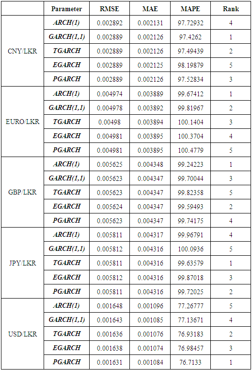
5. Conclusions

This paper investigated the comparison criteria between symmetric and asymmetric GARCH family models, based on the exchange rate volatility of the selected five top ranked economically stable countries with currency values of Chinese Yuan, Sterling Pound, Japan Yen, Euro and U.S.Dollars against Sri Lankan Rupees from the period of January 2010 to August 2018, which were extracted from Fred Online database. Exchange rates were used to evaluate the forecasting performance of the GARCH family models which include, ARCH, GARCH, TGARCH, EGARCH and PGARCH with the level of (1,1), differencing the symmetric and asymmetric effects. Normal (Gaussian) distribution is the only method, which was incorporated for the evaluation of data. It was attempted to very, how symmetric effects are influenced on positive or negative shocks towards the volatility responds to the global market fluctuations. Final result was concluded with the forecast estimate using RMSE, MAE and MAPE using selected in-sample data.