Ogunrinde R. B., Ayinde S. O.
Ekiti State University, Faculty of Science, Department of Mathematics, Ado Ekiti, Nigeria
Correspondence to: Ayinde S. O., Ekiti State University, Faculty of Science, Department of Mathematics, Ado Ekiti, Nigeria.
| Email: |  |
Copyright © 2018 The Author(s). Published by Scientific & Academic Publishing.
This work is licensed under the Creative Commons Attribution International License (CC BY).
http://creativecommons.org/licenses/by/4.0/

Abstract
In this research work, an interpolating function was proposed following Gompertz function approach and a Numerical Method was developed to solve problem in tumour growth analysis. Gompertz function or curve was for long of interest only to Actuaries and Demographics. It's, however, recently been used by various authors as a growth curve or function both for Biological, Economics and Management phenomena. Tumour are tiny cells developed from single cell to wider cells as the nutrients supply in the body is sufficient until it reached the carrying capacity.
Keywords:
Gompertz Function, Mathematical Method, Tumor growth, Carrying capacity
Cite this paper: Ogunrinde R. B., Ayinde S. O., Interpolating and Gompertz Function Approach in Tumour Growth Analysis, American Journal of Mathematics and Statistics, Vol. 8 No. 5, 2018, pp. 119-125. doi: 10.5923/j.ajms.20180805.03.
1. Introduction
Cancer is a wide range of diseases that has in common and unusual cells proliferation of the organism itself. It is an uncontrolled proliferation that provokes the formulation of a cellular mass named Tumor. For the tumor to develop beyond a given volume, it needs to develop the capacity to promote the growth of new blood vases towards itself. Those new vases well proportionate the blood irrigation of the tumor, supplying its needs of nutrition and oxygenation. [4].Heiko [6], submitted that the number of cancer cells in a tumor is difficult to estimate due to continuous changes in time. Tumor cells may proliferate, rest, in a quiescent state or die. Describing the numbers of tumor cells as a function of time which is therefore remarkably challenging. The number of living cells only changes when cells proliferate or die. However, difference in live cell number over time interval is equal the number of cells created and died over time interval. The basis of any mathematical model used to study cancer is a model of tumor growth. A number of Ordinary Differential Equation models (ODE) have been proposed to represent tumor growth and are regularly used to make predictions about the efficacy of cancer growth. Unfortunately, choice of a growth model is often driven by ease of mathematical analysis rather than whether it provides the best model for growth of a tumor.Some researchers have attempted to find the best ODE growth model by fitting various models to a small number of experimental data sets of tumor growth. Seven ordinary differential equation (ODE) models of tumor growth (exponential, Mendelsohn, logistic, linear, surface, Gompertz, and Bertalanffy) have been proposed, Taken altogether, the results are rather inconclusive, with results suggesting that choice of growth model depends at least in part on the type of tumor. This leaves modelers with little guidance in choosing a tumor growth model. [9].Among all seven of the previously proposed ODE models in the presence and absence of chemotherapy. We follow the suite of Gompertz Benjamin, derived an equation and used a sample data set to show how these quantities differ based on choice of growth model. Benjamin Gompertz originally created the Gompertz model in 1825 in order to explain human mortality curves [4], [5]. In 1938, The model became a generalization of the logistic model with a sigmoidal curve that is asymmetrical with the point of inflection [11]. The curve was eventually applied to model growth in size of entire organisms and more recently, was shown to provide the best fits for breast and lung cancer growth [1], [8].The Gompertz equation proposed and followed by [7] which form the basic equation applied in this paper is as follows: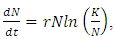 | (1) |
where  is the population of tumor cells. r is the constant intrinsic growth of cells, with
  K is the carrying capacity of the tumor, that is, the maximum size that it can achieve with the available nutrients. [10]. Based on the findings he generated the following facts that the carrying capacity, K, of a tumor be intimately related with quantity of tumors cells,
  and the value is
  cells, the rate
  , and
, and  where these values was used for Gompertz equation. [7].
2. Derivation of the Numerical Integration
2.1. Representation of Interpolating Function
A. Let us assume that the theoretical solution  to the initial value problem
 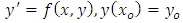 | (2) |
can be locally represented in the interval  by the non-polynomial interpolating function;
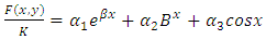 | (3) |
Where  are real undetermined coefficients,
  are the shape and scale parameters, K represent the saturation level using Gompertz approach. The intervals defined are
  and
and  . We shall assume
  is a numerical estimate to the theoretical solution
  and
and  .We define mesh points as follows:
 | (4) |
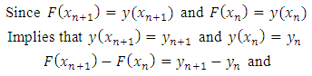
We can impose the following constraints on the interpolating function (3) in order to get the undetermined coefficients. [3]a. The interpolating function must coincide with the theoretical solution at  . Hence we required that
 | (5) |
and | (6) |
2.2. Derivatives of the Ordinary Differential Equation
The derivatives of the interpolating function are required to coincide with the differential equation as well as its first, second, and third derivatives with respect to  . [3] We denote the i-th total derivatives of
  with respect to x with
  such that
  | (7) |
This implies that,  | (8) |
 | (9) |
 | (10) |
These form a system of linear equation which can be solved using Cramer’s rule, hence solving for 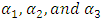 from the system of equation (8) to (10), we have
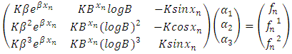 | (11) |
When taking (11) as a system of equations,  , it gives
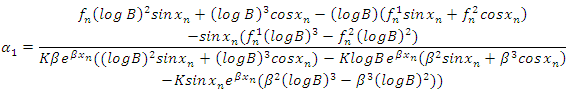 | (12) |
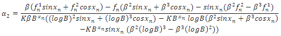 | (13) |
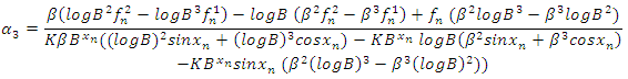 | (14) |
2.3. Formation of Numerical Integration
 | (15) |
Therefore, we shall have from (5) and (6) | (16) |
 | (17) |
 | (18) |
Therefore, by expansion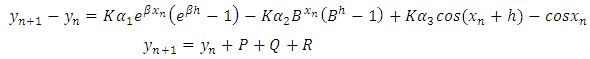 | (19) |
Where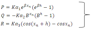 | (20) |
Substituting for  in (20), we have
 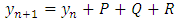 | (21) |
where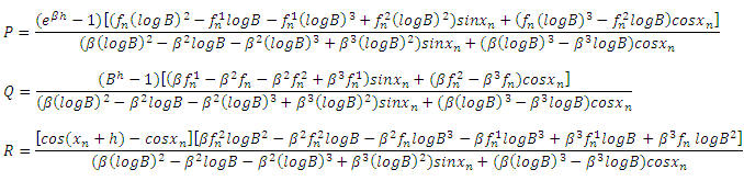 Equation (21) is the new numerical integration for solution of the first order differential equation. This numerical integration has been tested on some initial value problems of first order differential equations [12].
3. Implementation of the Integration to Solve Tumor Growth Problem
The Gompertz equation was developed in 1938. He used it to describe the growth of solid tumor assuming that the growth rate of tumors diminishes in a non – linear way when its mass increase.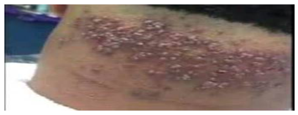 | Picture 1. Skull/Skin Tumor (Source: www.google/skull tumor) |
As it was used by [7], the rate r is invariable, the equation is better represented as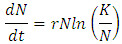 Where
Where  is the population of tumor cells.r is the constant intrinsic growth of cells, with
  K is the carrying capacity of the tumor, that is, the maximum size that it can achieve with the available nutrients. [10]Problem 1: TUMOR GROWTH [2]The carrying capacity, K, of a tumor be intimately related with quantity of tumors cells,
  and the value is 1013 cells, the rate
  , and
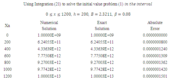
, and  With the parameter given above, find the variation rate of the tumor cell population if (i) the cycles of timing evolution is 0 to 1200.(ii) the cycles of timing evolution is 0 to 600.Using the Numerical Integration (21) also known as Numerical Method, we have SOLUTION
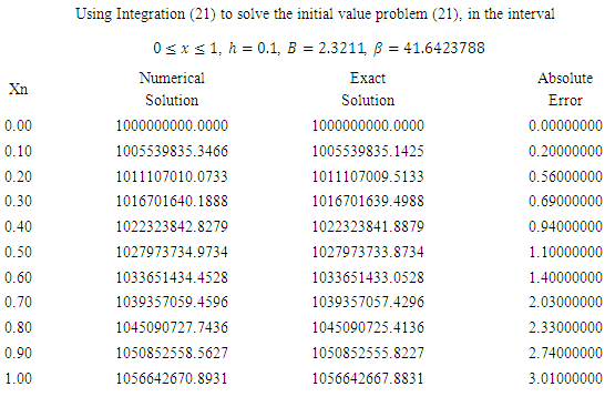
Table 1. Results of Problem 1, population of Tumour cells
 |
| |
|
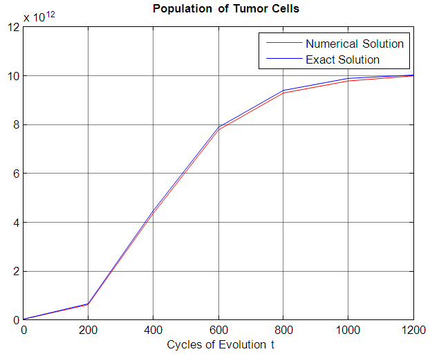
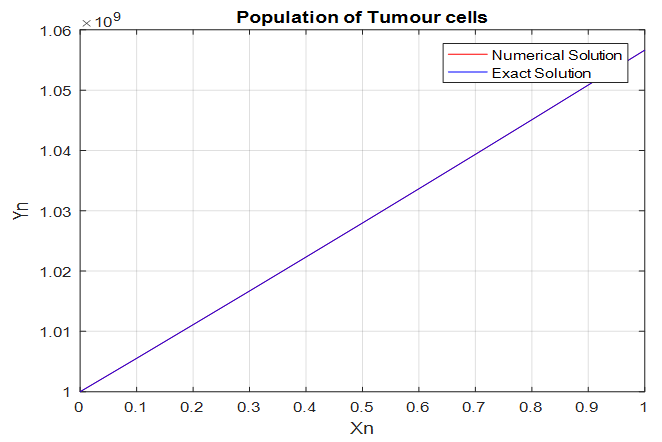 | Figure 1. The graph of the Numerical and Exact solution of 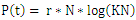 . For the variation rate of the tumor cell population growth . For the variation rate of the tumor cell population growth |
(i) The variation rate of the tumor cell population if the cycles of timing evolution is 0 to 1200.Table 2. Results of Problem 1, population of timing evolution is 0 to 1200
 |
| |
|
 | Figure 2. The graph of the Numerical and Exact solution of 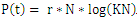 . The variation rate of the tumor cell population if the cycles of timing evolution is 0 to 1200 . The variation rate of the tumor cell population if the cycles of timing evolution is 0 to 1200 |
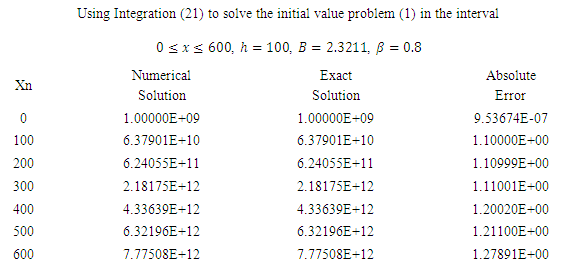
(ii) The variation rate of the tumor cell population if the cycles of timing evolution is 0 to 600.Table 3. Results of Problem 1, population of timing evolution is 0 to 600
 |
| |
|
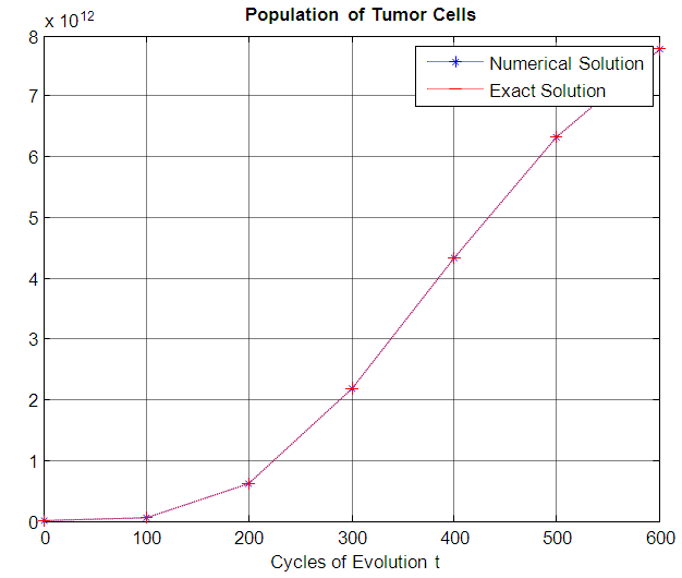 | Figure 3. The graph of the Numerical and Exact solution of 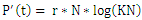 . The variation rate of the tumor cell population if the cycles of timing evolution is 0 to 600 . The variation rate of the tumor cell population if the cycles of timing evolution is 0 to 600 |
4. Discussion
Looking at the three tables showing above, though,  , which is fixed as a result of the carrying capacity, the difference in
  and
and  clearly indicates that the Tumour growth varies from stage to stages, and rate of proliferation cannot be fixed any way, In table 1, the blue colour indicating the exact solution suppress the red colour of numerical solution showing the effectiveness of the numerical integration.
5. Conclusions
As increasing variety of mathematical models has made its way into cancer research over the past decades especially in Tumour growth problem, little is done on using numerical integration to solve this problem. In this research work, we have illustrated how quantitative models in term of interpolating function can be developed and analyzed into numerical integration, and used experimental data to show how it can simulate complex biological processes in Tumour growth. The results obtained in numerical solution is comparably with the exact solution which showed the effectiveness of the method.Moreover, the Logistic model or equation used in this analysis as well as Gompertz equation can be modified as its being done by many analysists. The case of nutrient and treatment is however, suppressed.
List of Abbreviations
Ordinary Differential Equations (ODE).
ACKNOWLEDGEMENTS
I want to appreciate the efforts of my Ph.D supervisors, Prof. Ibijola E. A. and Dr. (Mrs) Ogunrinde R. B.
References
| [1] | Benzekry S., Lamont C., Beheshti A., Amanda T., John M. L., Hlatky L., Hahnfeldt P. (2014). “Classical Mathematical Model for Description and Prediction of Experimental Tumor Growth.”. Plos Computational Biology. Open Access. 10(8): 1003800. |
| [2] | Domingues, J. S. (2010). “Modelo Matemático e Computacional do Efeito do Surgimento da Angiogênese em Tumores e sua Conexão com as Células Tronco.” CEFET – MG. Dissertac̡ão de Mesterdo, Brasil. |
| [3] | Fatunla, S.O. (1988). “Numerical Methods for Initial Value Problems in Ordinary Differential Equations”. Academic Press, San Diego, USA. |
| [4] | Gompertz, B. (1825). “On the Nature of function Expressive of the Law of Human Mortality and on a new mode of determine the value of life contingencies”. Philosophical Transaction of the Royal Society of London. 115: 513583. |
| [5] | Gompertz, B. (1860). “On one Uniform Law of Mortality from birth to extreme old age and on the Law of Sickness” presented to internal Statistical congress in 1860 and reported in 1871. Journal of the Institute of Actuaries. 16, 329 – 344. |
| [6] | Heiko, E. and Mark, A.J. (2014). “Mathematical Modeling of Tumor Growth and Treatment”. Current Pharmaceutical Design. 20,000-000. ISSN: 1381-6128. |
| [7] | Jose, S.D. (2012). “Gompertz Model: Resolution and Analysis for Tumors”. Journal of Mathematical Modelling and Application. Vol. 1, No. 7. 70 – 77. ISSN: 2178-2423. |
| [8] | Mehrara E., Forsell A. E., Johanson V., Koolby L., Hultborn R., Bernhardt P. (2013). “A new method to estimate parameters of the growth model for metastatic Tumors.” Theoretical Biology Medical Model. 10: 31-43. doi:10.1186/1742-4682-10-31. |
| [9] | Murphy, H., Jaafari, H., Dobrovolny, H. M. (2016). “Differences in Predictions of ODE Models of Tumor Growth: a cautionary example”. BioMedCentral. Cancer. Open Access. 16:163. |
| [10] | Sachs, R., Hlatky, L. R., Hahnfeldt, P., (2001). “Simple ODE Models of Tumor Growth and Anti-Angiogenic or Radiation Treatment.” PERGAMON – Mathematical and Modelling. 33, 1297 – 1305. |
| [11] | Winsor, C.P. (1932). “The Gompertz Curve as a Growth Curve”. Proceedings of the National Academy of Sciences. USA. Vol 18, No 1, 1-8. |
| [12] | Ogunrinde R. B., and Ayinde S. O. (2017). “A Numerical Integration for Solving First Order Differential Equation Using Gompertz Function Approach”. American Journal of Computational and Applied Mathematics. 7(6): 143 – 148. |

 Abstract
 Reference
 Full-Text PDF
 Full-text HTML