-
Paper Information
- Next Paper
- Paper Submission
-
Journal Information
- About This Journal
- Editorial Board
- Current Issue
- Archive
- Author Guidelines
- Contact Us
American Journal of Mathematics and Statistics
p-ISSN: 2162-948X e-ISSN: 2162-8475
2018; 8(5): 105-110
doi:10.5923/j.ajms.20180805.01

Efficiency of Some Estimation Methods of the Parameters of a Two-Parameter Pareto Distribution
 Abstract
 Reference
 Full-Text PDF
 Full-text HTML
Emmanuel John Ekpenyong1, Okechukwu J. Njoku1, Victoria M. Akpan2
1Department of Statistics, Michael Okpara University of Agriculture, Umudike, Nigeria
2Department of Statistics, Akwa Ibom State Polytechnic, Ikot Osurua, Nigeria
Correspondence to: Emmanuel John Ekpenyong, Department of Statistics, Michael Okpara University of Agriculture, Umudike, Nigeria.
| Email: |  |
Copyright © 2018 The Author(s). Published by Scientific & Academic Publishing.
This work is licensed under the Creative Commons Attribution International License (CC BY).
http://creativecommons.org/licenses/by/4.0/

This work considered the estimation of the parameters of a two-parameter Pareto distribution. Four methods of estimation namely, the Methods of Moments (MM), Methods of Maximum Likelihood (MLE), Methods of Least Squares (OLS) and Ridge Regression (RR) method were employed to estimate the parameters of the distribution. One thousand (1000) random variables that followed the distribution of the two-parameter Pareto distribution with the shape parameter, (β=5) and scale parameter (α=10) were simulated using the R statistical software. Different samples of sizes 20, 40, 60 and 80 were drawn from the simulated population repeatedly for about 100 times and the parameters of the distribution estimated using the specified methods. The estimated parameters were used in each case to fit the estimated cumulative distribution function. These estimated parameters for each method were compared using the measures of Total Deviation (TD) and the Mean Square Error as the goodness of fit criteria. Results showed that the method of Maximum likelihood was found to give the best fit and this was followed by the Ordinary Least Squares (OLS) method. On the whole, the methods seemed to give consistent estimators as the estimated parameters approached the original parameters as the sample size increased.
Keywords: Two-parameter Pareto Distribution, Estimation methods, Goodness of fit, Ridge regression, Maximum likelihood methods, Ordinary least squares, Method of moments
Cite this paper: Emmanuel John Ekpenyong, Okechukwu J. Njoku, Victoria M. Akpan, Efficiency of Some Estimation Methods of the Parameters of a Two-Parameter Pareto Distribution, American Journal of Mathematics and Statistics, Vol. 8 No. 5, 2018, pp. 105-110. doi: 10.5923/j.ajms.20180805.01.
Article Outline
1. Introduction
- Distribution fitting has been of great importance in different areas of science. It is used to select a model (statistical distribution) which best describes the pattern (fits) of a dataset generated by some random process. The advantage of distribution fitting to data is that it allows for the development of valid models of random process and by so doing gives possibilities for proper predictions of future occurrences which in turn help in making better decisions. The challenge faced in distribution fitting is obtaining the model with the best fit. This includes getting the method of estimation which is most efficient, the appropriate probability distribution, the appropriate goodness of fit criterion to compare the efficiency of the model and nature of the data. The Pareto distribution is one of such statistical distribution where such challenges are faced. The Pareto distribution is a power law probability distribution that is used in modeling many observable phenomena in description of social, scientific, geophysical, and actuarial science. It has been widely applied in the area of economics, trade, Insurance, Meteorology, Business and social sciences to model some real life phenomena. This has been showcased in the works of Nursamsiah et al. (2018), Ghitany et al. (2018) and Amand et al. (2016). There is a wide range of situation where the choice of the model can be made focusing just on the specific task to be accomplished while inaccuracy in unimportant areas is wittingly accepted. Nevertheless, sometimes the challenge is not on the choice of the model but the method of estimation or fitting the model. Such cases may arise in the Pareto distribution when the data is too heavy-tailed or having outliers or extreme values or when the sample sizes are small. The challenge in such cases is not just to choose a model but to find a robust and most appropriate method of fitting the distribution to the data.There is a hierarchy of Pareto distributions known as Pareto Type I, II, III, IV, and Feller–Pareto distributions (Barry, 1983; Johnson et al., 1994). Burroughs and Tebbens (2001a) estimated parameters of the truncated Pareto distribution by least squares fitting on a probability plot while Burroughs and Tebbens (2001b) minimized the mean squared error fit on a plot of the tail distribution function). Beg (1981) also provided maximum likelihood estimates of the lower truncation parameter, scale, and probability of exceedance for a truncated Pareto distribution. The maximum likelihood estimator (MLE) of the scale parameter (α) when the lower truncation limit is known was presented by Cohen and Whitten (1988), with some recommendations for the case when the lower truncation limit is not known. vanZyl (2015) showed that random variables of the generalized three-parameter Pareto distribution can be transformed to that of the Pareto distribution. They tested the performance of the estimation of the shape parameter of generalized Pareto distribution using transformed observations and their results indicated that it improved the performance with respect to relative efficiency. Quandt (1966) used the Method of Moments (MOM), while Baxter (1980) and Cook and Mumme (1981) used the method of Maximum Likelihood Estimation (MLE) for the Pareto distribution. vanMontfort and Witter (1986) used the MLE to fit the Generalized Pareto distribution to represent the Dutch POT rainfall series and used an empirical correction formula to reduce bias of the scale and shape parameter estimates. Kim et al. (2017) proposed a new parameter estimator that utilizes a pivotal quantity based on the regression framework, allowing separate estimation of the two parameters in a straightforward manner. They affirmed that the method has the ability of overcoming the limitation of the Maximum Likelihood estimation method. Dalpatadu and Singh (2015) attempted to estimate the parameters of a two-parameter Pareto distribution using a Minimization Technique of a distance function such as the Kolmogorov-Smirnov distance with the help of the Golden Search procedure. They showed that the method was fairly simple and accurate and may be improved using a larger sample; but the work did not compare the method with existing estimation methods. Other authors estimated the parameters of a Generalized Pareto Distribution (GPD) using various methods (see Oztekin, 2005; Hosking et al., 1987). Bhatti et al. (2018a) however proposed three modified percentiles estimators of the parameter of a two-parameter Pareto distribution. They based their modifications on median, geometric mean, and expectation of empirical cumulative distribution function (CDF) of the first-order statistic. The proposed estimators were compared with the traditional percentile estimators through a Monte Carlo simulation. Results showed that the proposed estimators provided efficient and precise parameter estimates that the traditional percentile estrimators considered. Also, Zaher et al (2014) obtained the Fuzzy Least Squares estimator for the two-parameter Pareto distribution and compared it with the different methods of nestimation – the Trimmed Linear moments (TL-moments), Linear moments (L-moments) and Linear Quantile moments (LQ-moments). It was shown that the proposed Fuzzy Least Squares estimator was preferable at all times. Bhatti et al. (2018b) proposed some modifications in the maximum likelihood estimation methods of a Pareto distribution and evaluated their performances. They discovered that the modified maximum likelihood estimators based on expectation of empirical cumulative distribution function (CDF) of first order statistic performed much better than the traditional maximum likelihood estimator and other modified estimators on median and coefficient of variatiion. Hussain et al. (2018) also proposed four modified moment estimators for the parameter of the Pareto distribution. These estimators were compared with the traditional method of moments. The modified moment estimators based on mean of first order statistics and expectation of empirical cumulative distribution function of first order statistics were demonstrated to perform better than the traditional estimator and other modified moment estimators. In the same vein, Zaka et al. (2013) considered modifications of maximum likelihood, moments and percentile estimators of a two-parameter Poareto distribution. They concluded that for some combinations of parameter values, some of the modified traditional maximum likelihood, moments and percentile estimators in terms of bias, mean square error and total deviation. However, this work seeks to estimate the parameters of a two-parameter Pareto distribution to simulated data using some methods of estimation (Method of Moments, Maximum Likelihood method, Least Squares Methods and Ridge Regression Method) at different samples sizes, and to compare the fits by these methods of estimation using some goodness of fit criteria.
2. Methods of Analysis
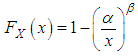
2.1. Estimating Parameters of a Two-parameter Pareto Distribution
- The two-parameter Pareto distribution (also called the Type I Pareto distribution) can be defined in terms of its cumulative distribution function as:
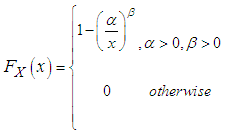 | (3.1) |
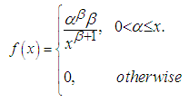 | (3.2) |
2.1.1. Method of Moments (MOM)
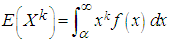
- By definition (1.5), the kth moment of the Pareto distribution is given as:
 In order to obtain the estimate of
  from a sample of n observations, we recall that the probability of an observation greater than x is
  . Thus, the probability that all n sample values
  are greater than x is
  . This is, therefore also the probability that the lowest sample value is greater than x.Thus, the c.d.f of the lowest sample is
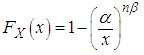 | (3.3) |
 | (3.4) |
 | (3.5) |
 is the minimum value and
  is the mean.
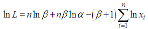
2.1.2. Method of Maximum Likelihood (MLE)
- Given that
 are random variables that follow the Pareto distribution, the likelihood function denoted by
  for the sample is:
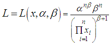 | (3.6) |
 | (3.7) |
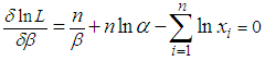 | (3.8) |
 the subject formula, we have:
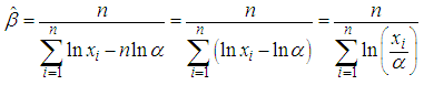 | (3.9) |
 | (3.10) |
 | (3.11) |
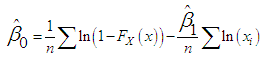
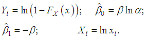
2.1.3. Least Squares Method (LSE)
- For the estimation of probability distribution parameters, the least squares method (LSM) is extensively used in reliability engineering and mathematics problems.Given that the cumulative density function of the Pareto distribution is given as:
 | (3.12) |
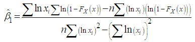 | (3.13) |
 | (3.14) |
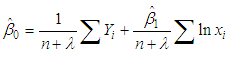
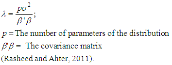
2.1.4. Ridge Regression Method (RR)
- Like the method of LSE, the ridge regression estimates of
 and
and  can be obtained by minimizing the error sum of square for the model:
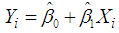 subject to the single constraint that
  , where
  is a finite positive constraint. Using the method of Lagrange's multiplier, we obtain:
 | (3.15) |
 | (3.16) |
 | (3.17) |
 | (3.18) |
2.2. Goodness of Fit Tests
- AL-Fawzan (2000) referred to the use of the procedure of MSE and TD as a goodness of fit test.
2.2.1. Mean Square Error (MSE)
- The MSE can be calculated using the formula below:
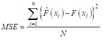 | (3.19) |
 is the value of the cumulative distribution function of the two-parameter Pareto distribution using the estimated parameters, and
  is the empirical cumulative distribution function. (Rasheed and Ahter, 2011).
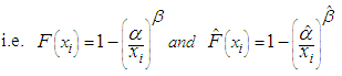
2.2.2. Total Deviation (TD)
- The total deviation TD can be calculated for each method as:
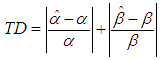 | (3.20) |
 and
and  are the estimated parameters by any method.The method with the minimum total absolute deviation would be selected as the most efficient parametric method for fitting the distribution or estimating the parameters.
3. Results and Discussion
3.1. Results
- The data used for evaluating the adequacy of the methods of estimating the parameters of the Pareto distribution (fitting the Pareto distribution) is a simulated data from R. In the simulation, 1000 random numbers that follows a pareto distribution of shape parameter (β=5) and scale parameter (α=10) were generated. Different samples of sizes 20, 40, 60 and 80 were drawn from the simulated population repeated for about 100 times and their respective fits were estimated.Figure 1 indicates the plot of the two-parameter Pareto density function with shape parameter, β=5 and Location parameter, α =10. From the figure, it is observed that the function tails heavily to the right. This is one of the properties of the Pareto distribution.
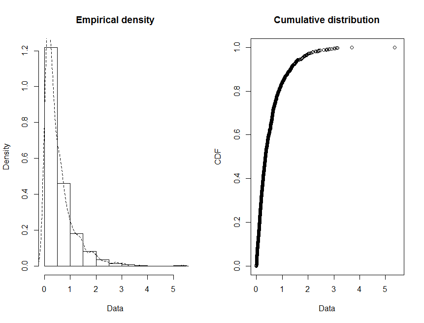 | Figure 1. Density plot and Cumulative distribution plot for shape = 5, scale = 10 |
|
3.2. Discussion of Results
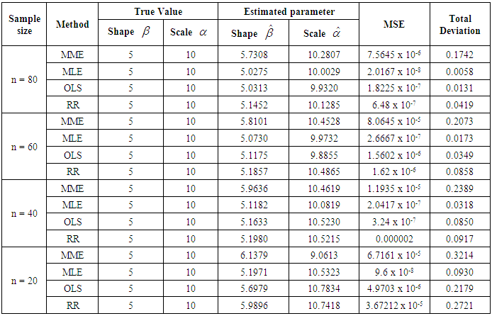
- From Table 1, the Maximum Likelihood Estimator was identified as the most efficient estimator because it gave the least MSE and TD for all sample sizes considered in this work. This agrees with the work of Witter (1986) where MLE proved to be the most efficient method to fit the generalized Pareto Distribution to represent the Dutch POT rainfall series. This was followed by the method of ordinary least squares. The maximum likelihood estimator and the method of ordinary least squares have been known to be consistent estimators. These have been proven mathematically by Quandts (1964).
4. Conclusions
- Based on the results obtained from this study, we have sufficient evidence to conclude that the Maximum Likelihood Estimation method is a more adequate method for fitting the two-parameter Pareto distribution when the series is free of outliers. The maximum likelihood estimator has also proven to be the most efficient estimator above the method of moment, ordinary least square estimator and the ridged regression estimator. It is also observed from the analysis that all methods seemed to be consistent in estimating the parameters.