-
Paper Information
- Paper Submission
-
Journal Information
- About This Journal
- Editorial Board
- Current Issue
- Archive
- Author Guidelines
- Contact Us
American Journal of Mathematics and Statistics
p-ISSN: 2162-948X e-ISSN: 2162-8475
2018; 8(4): 99-104
doi:10.5923/j.ajms.20180804.04

On the Extension of the Mover-Stayer Model when Rate of Transition Follows Negative Binomial Distribution
 Abstract
 Reference
 Full-Text PDF
 Full-text HTML
Adams Y. J., Abdulkadir S. S.
Modibbo Adama University of Technology, Yola, Nigeria
Correspondence to: Adams Y. J., Modibbo Adama University of Technology, Yola, Nigeria.
| Email: |  |
Copyright © 2018 The Author(s). Published by Scientific & Academic Publishing.
This work is licensed under the Creative Commons Attribution International License (CC BY).
http://creativecommons.org/licenses/by/4.0/

The extension of the Mover-Stayer Model proposed by Blumen, Kogan and McCarthy (1955) is an active area of research. Spilerman (1972) extended the basic model by specifying gamma distribution for the transition rate, the mixture of which resulted in Negative Binomial distribution. However, the Negative Binomial distribution being a unimodal distribution, may not capture situations where excess zeroes exist in the distribution of movements. This paper extends the model using Negative Binomial distribution to model rate of transition in Poisson distribution, which gave the Polya-Aeppli distribution (which is bimodal) as a mixture. The obtained model was validated using a simulated data adopted from Spilerman (1972).
Keywords: Mover-Stayer, Polya-Aeppli, Negative Binomial, Bimodal
Cite this paper: Adams Y. J., Abdulkadir S. S., On the Extension of the Mover-Stayer Model when Rate of Transition Follows Negative Binomial Distribution, American Journal of Mathematics and Statistics, Vol. 8 No. 4, 2018, pp. 99-104. doi: 10.5923/j.ajms.20180804.04.
Article Outline
1. Introduction
- Markov chain model has a wide range of applications in social mobility. The model requires assumptions of stationarity and population homogeneity, that is, every element (individual) has the same probability of moving, say, from state i to state j, and the movement (transition) conditioned only on the state in the immediate previous time period. But transition from an origin state hardly conform to this assumption (Spilerman, 1972). However, Blumen, Kogan, and McCarthy, (1955) noted in their interesting study of the movement of workers among various industrial aggregates in US that some individuals simply move more often than, or differently from, others. This idea was also found in the study with intergeneration and intragenerational occupational mobility (Hodge, 1966; Lieberson and Fuguitt, 1967), and with geographical migration (Rogers, 1966; Tarver and Gurley, 1965). This principle led to introduction of heterogeneity to the transition (movement) of an individuals in the population during a unit interval. This idea introduces heterogeneity to the transition (movement) of individuals in the population during a unit interval. With the assumption of heterogeneity, all individuals move according to an identical transition when they move but differ in their rate of mobility. Hence this has resulted to development of “mover-stayer” model (Blumen, Kogan, and McCarthy, 1955, Spilerman, 1972). This implies two types of individuals: the stayer, who with probability one remains in the same category during the entire period of study and the ‘mover ‘whose changes in category overtime can be described by a Markov chain with constant probability matrix. The model is appropriate for the analysis of geographical migration or intragenerational occupation mobility where repeated moves can be made by a person. Spilerman (1972) observed that most of mobility data lacks significant detail at the individual level, the mover-stayer model can be applied where the construction of sub-population transition matrices is not possible. Goodman (1961) noted that the transition probability matrix for movers, and the proportion of stayers among the individuals in each category at, say, the initial point in time, are unknown; the estimators provided by BKM for the stayer-movers are inconsistent. There is a lot of estimation methods that have been provided in literatures (Goodman, 1960, Liu and Chen, 2015; Morgan, Aneshensel, and Clark, 1983). Frydman (1984) obtained the maximum likelihood estimation of the mover-stayer model’s parameters by direct maximization of the likelihood, while Fuchs and greenhouse (1988) provided expected –maximization (EM).This paper is motivated by the statement made in Spilerman (1972) that the originators of mover-stayer model, Blumen, Kogan, and McCarthy (BKM), discuss strategies for extending the mover-stayer model to incorporate a wider range of heterogeneity in the rate of transition, but they do not develop such generalization. BKM proposed in their method of generalization of mover-stayer that instead of postulating two types of persons, we should extent to a process which handle several types. They argue that relaxation of fixed number of movement assumption does not prevent the population process-level from being Markovian and cited the example where transitions are Poisson events and the population is homogeneous in its transition rate, the Markov requirement will be appropriate. It is on this basis that Spilerman (1972) extend the basic model by specify a distribution for the transition rate to follow gamma distribution. That is, he assumes Poisson process transition and its rate to follow gamma distribution which resulted in Negative binomial distribution. His reasoning for the choice is that there is little prior knowledge about its (i.e. rate) distribution. However, gamma is unimodal and may not capture situation where the mobility data consist of multi-modal. In literature different distributions have been suggested to model the rate of movement (or random effect). For instance, O’Keefe et.al (2012) in their study of psoriatic arthritis consider gamma, inverse Gaussian(IG), and Compound Poisson distribution(CP) for random effects in mover-stayer multistate models. Yiu, Farewell and Tom (2016) explore the existence of a stayer population with mover-stayer counting process model on joint damage, gamma, inverse Gaussian and compound Poisson were considered for random-effects. Cook et.al (2002) developed a generalized mover-stayer model for panel data where an individual is allows to move among states according to the underlying Markov process until it encounters one of its absorbing states, where he can no longer move.
2. Methodology
2.1. The Mover – Stayer Model
- In the mover-stayer first proposed by Blumen and associates (1955), it is noted that the computations of k-step transition matrices from Markov chain consistently underpredicts the main diagonal elements of the observed k-step matrix. That is,
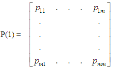 Where P(1) is the observed one- step transition matrix, and P(k)
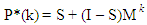
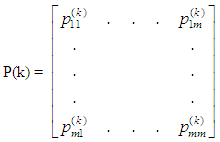 is the observed k-step transition matrix. If the P*(k) is predicted using Markov process, the diagonal elements of the predicted transition matrix will be less than the elements in the observed k-step transition matrix. The reason for the inequality in diagonal elements of the two matrices was attributed to some individuals move more often than others, for each time interval, hence BKM suggested decomposition of the matrix into two subpopulations: the movers and the stayers, because some persons are less apt to move than others in each time interval,
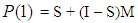 | (1) |
 | (2) |
 . This is given by
 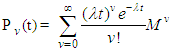 | (3a) |
 is the transition matrix in the interval (0, t). For t =1 equation (3a) becomes
  Where
Where | (3b) |
 | (4) |
 is the proportion of the ith subpopulation who move with rate
  , and if the sampling is made from a continuous distribution
  , we obtain
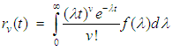 | (5) |
 to obtain negative binomial distribution. That is,
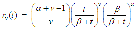 | (6) |
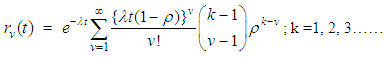
 . The choice of the negative binomial as a mixing distribution is informed by considering the number of transitions required to achieved desire events
 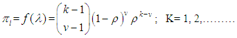 | (7) |
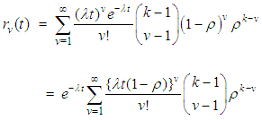 | (8) |
 | (9) |
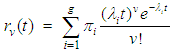
 the distribution in (9) reduces to the classical homogenous Poisson distribution (Minkova, 2002; Minkova, 2004; Chukova and Minkova, 2012). The Polya-Aeppli distribution often called the Inflated-Parameter Poisson [IPo(λ, ρ)] is defined as follows (Minkova & Balakrishnan, 2014). We define the number of transitions made before the number of required event as N(t) in the interval (0,t) ,where N(t) is
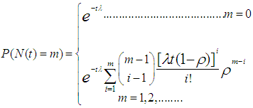 | (10) |
 | (11) |
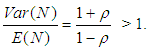 Therefore, not only Poisson process is a particular case of Pólya-Aeppli process, but for
  the Pólya-Aeppli process is over-dispersed, which provides a greater flexibility in modeling count data than the standard Poisson process (Chukova & Minkova, 2012).In general, the Neyman Type A and Thomas distributions can have any number of modes from one upwards. The Pólya-Aeppli distribution, on the other hand, has either one or two modes, while the negative binomial has always one mode (Ascombe, 1950).The most commonly used distribution to model overdispersed data is the negative binomial, but other distributions may be more appropriate for modelling data with excess zeros, because, unlike the negative binomial, they can have more than one mode, including a mode at zero. Examples include the Neyman Type A and Pólya-Aeppli distributions (Ridout et. al, 1998).
3. Parameter Estimation and Model Validation
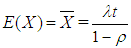
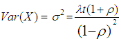
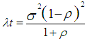
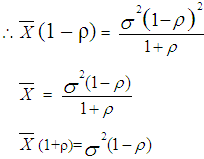
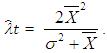
3.1. Moment Estimates of λt and ρ of the Polya-Aeppli Distribution
 | (12) |
 | (13) |
 | (14) |
 | (15) |
 | (16) |
 | (17) |
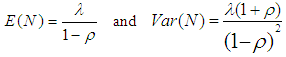
 Therefore, the remaining parameters of the model
  of the Polya Aeppli distribution, can be estimated directly from observed data on the number of moves by an individual. If
  and
and  are the sampling mean and variance of this variable (number of moves), then estimates of
  can be obtained in terms of these values (see also Minkova, 2012, p. 49). This yields
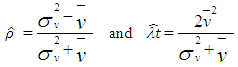 | (18) |
 and
and  from the observed data.
3.2. Testing the Model with Simulated Data
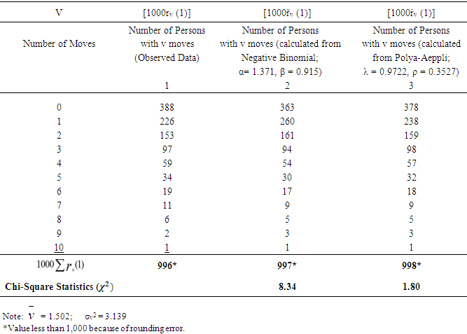
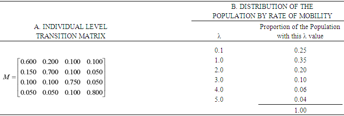
- In order to validate the proposed model, we adopt the structure of the simulated data as provided by Spilerman, 1972 (p. 610), where in the absence of full knowledge of the actual mobility characteristics of the hypothetical population, individual level transition matrix and a population distribution by rate of movement is presented by assuming six types of persons in the population who move in accordance with Poisson process specified by λ = 0.1, 1.0, 2.0, 3.0, 4.0 and 5.0, while the states of the process defined by four geographic regions, given rise to a 4x4 transition matrix (Table 1). The Poisson distribution was used to generate an expected proportion of each subpopulation who make v = 0, 1, 2,…. moves during the time interval (0,1). These values, multiplied by their respective subpopulation proportions in the total population, were aggregated to produce a distribution of the total population by number of moves. In this case the Poisson estimates were considered as the observed data, and the expected frequencies generated using negative binomial and Polya – Aeppli distributions, and comparison were made among the three distributions using Chi-square as Goodness of fit test. Out of the three distribution, Polya-Aeppli has the smallest chi-square.
|
4. Discussion and Conclusions
- The Poisson distribution model was used as a baseline model to generate individual level transition matrix and the observed frequency distribution of moves. The expected frequencies were obtained using Polya-Aeppli distribution.The comparison of the observed frequencies in column 1 of Table 2 with the expected values given in columns 2 and 3 of the same table, shows that Polya-Aeppli distribution fits the observed frequencies much better than the negative binomial distribution which was proposed by Spilerman (1972). The value of
 is 1.80 as against tabular value of 14.067 which shows that the approximation by Polya-Aeppli distribution is acceptable.
|