Deapon Biswas
Transport Officer, Private Concern, Chittagong, Bangladesh
Correspondence to: Deapon Biswas, Transport Officer, Private Concern, Chittagong, Bangladesh.
| Email: |  |
Copyright © 2018 The Author(s). Published by Scientific & Academic Publishing.
This work is licensed under the Creative Commons Attribution International License (CC BY).
http://creativecommons.org/licenses/by/4.0/

Abstract
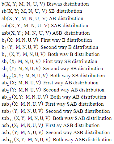
Here we get all the theoretical discrete distributions to the random experiment “M sided N dice taken V at a time”. It states joint probability functions as well as marginal probability functions of which number of possible outcomes is EB numbers and number of favorable outcomes is GB numbers. In this paper I introduce 20 definitions where first is the Biswas distribution and others are the related distributions that state different joint probability functions and marginal probability functions.
Keywords:
Biswas distribution, SB distribution, AB distribution, SAB distribution, ASB distribution, First way B distribution, Second way B distribution, Both way B distribution, First way SB distribution, Second way SB distribution, Both way SB distribution, First way AB distribution, Second way AB distribution, Both way AB distribution, First way SAB distribution, Second way SAB distribution, Both way SAB distribution, First way ASB distribution, Second way ASB distribution, Both way ASB distribution
Cite this paper: Deapon Biswas, Biswas Distribution, American Journal of Mathematics and Statistics, Vol. 8 No. 4, 2018, pp. 89-95. doi: 10.5923/j.ajms.20180804.02.
1. Introduction
First of all Biswas distributions are divided into four parts i.e., (i) both way selected B distribution (SB distribution)(ii) both way arranged B distribution (AB distribution)(iii) first way selected and second way arranged B distribution (SAB distribution)(iv) first way arranged and second way selected B distribution (ASB distribution)And then each part divided into three parts again i.e., for B distribution we get (i) first way B distribution(ii) second way B distribution (iii) both way B distribution.
2. Findings
Definition 3.1 Biswas distribution: A two dimensional random variable (X, Y) is said to follow Biswas distribution if it assumes only non negative values and its joint probability mass function is given by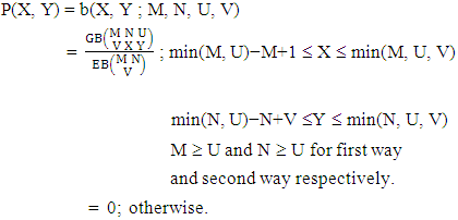 | (3.1) |
The four independent finite constants M, N, U and V are known as the parameters of this distribution. Biswas distribution is a joint probability distribution and a theoretical discrete distribution. Here X takes only non-negative values under the interval min(M, U)−M +1 ≤ X ≤ min(M, U, V) and Y takes only non-negative values under the interval min(N, U)−N+V ≤ Y ≤ min(N, U, V). Any two dimensional random variable which follows B distribution is known as B-variate and denoted by the symbol (X, Y) ∼ B(M, N, U, V).Remark: It should be noted that  | (3.2) |
Example 3.1: For the GB experiment  find P(X = 2, Y = 1) where the experiment is first way arranged and second way selected.Solution: We know
  Definition 3.2 SB distribution: A two dimensional random variable (X, Y) is said to follow SB distribution if it assumes only non-negative values and its joint probability mass function is given by
 | (3.3) |
Remark: It should be noted that  | (3.4) |
Example 3.2: For the GSB experiment  find (i) P(X =2, Y=3) and (ii) P(X=3,Y=1).Solution: We get
 Definition 3.3 AB distribution: A two dimensional random variable (X, Y) is said to follow AB distribution if it assumes only non-negative values and its joint probability mass function is given by
 | (3.5) |
Remark: It should be noted that  | (3.6) |
Example 3.3: For the GAB experiment  find (i) P(X=1,Y=3) and (ii) P(X=2,Y=2).Solution: We get
 Definition 3.4 SAB distribution: A two dimensional random variable (X, Y) is said to follow SAB distribution if it assumes only non-negative values and its joint probability mass function is given by
  | (3.7) |
Remark: It should be noted that  | (3.8) |
Example 3.4: Given the following favorite probability distribution of the experiment  .
.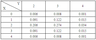 Find the probability of getting (i) X = 0, Y = 2, (ii) X = 2, Y = 3 and (iii) Y = 4.Solution:
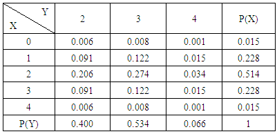 We get from the above table(i) Probability of getting X = 0, Y = 2 i.e., P(X = 0, Y = 2) = 0.06(ii) Probability of getting X = 2, Y = 3 i.e., P(X = 2, Y = 3) = 0.274 (iii) Probability of getting Y = 4 i.e., P(Y = 4) = 0.066.Definition 3.5 ASB distribution: A two dimensional random variable (X, Y) is said to follow ASB distribution if it assumes only non-negative values and its joint probability mass function is given by
 | (3.9) |
Remark: It should be noted that  | (3.10) |
Example 3.5: Given the following bivariate probability distribution of the experiment  .
.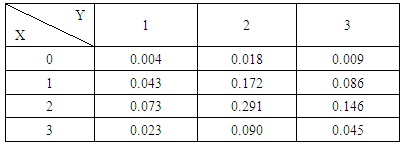 Find (i) P(X ≥ 2), (ii) P(X = 0, Y = 3), (iii) P(X ≤ 2, Y = 2) and (iv) P(X = 3, Y ≥ 2).Solution:
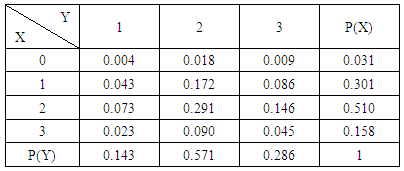 Solution: We get from the above table (i) P(X ≥ 2) = P(X = 2) + P(X = 3) = 0.510 + 0.158 = 0.668(ii) P(X = 0, Y = 3) = 0.009(iii) P(X ≤ 2, Y = 2) = P(X = 0, Y = 2) + P(X = 1, Y = 2) + P(X= 2, Y= 2) = 0.018 + 0.172 + 0.291 = 0.481 (iv) P(X = 3, Y ≥ 2) = P(X = 3, Y = 2) + P(X = 3, Y = 3) = 0.090 + 0.045= 0.135Now we describe three kinds of B distributions i.e., first way B distribution, second way B distribution and both way B distribution and their different forms. Definition 3.6 First way B distribution: Let the joint distribution of two random variables X and Y is given then the first way B distribution can be written as
 | (3.11) |
Remark: It should be noted that 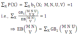 | (3.12) |
The first way B distribution is also known as the marginal probability distribution of X.Example 3.6: Given the following bivariate probability distribution of example 3.4 find first way B distribution of (i) X = 0 and (ii) X = 2.Solution: From the given table we get (i) P(X = 0) = 0.015 and (ii) P(X = 2) = 0.514.Definition 3.7 Second way B distribution: Let the joint distribution of two random variables X and Y is given then the second way B distribution can be written as | (3.13) |
Remark: It should be noted that 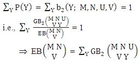 | (3.14) |
The second way B distribution is also known as the marginal probability distribution of Y. Example 3.7: Given the following bivariate probability distribution of example 3.4 find second way B distribution of (i) Y = 2 and (ii) Y = 4.Solution: From the given table we get (i) P(Y = 2) = 0.400 and (ii) P(Y = 4) = 0.066.Definition 3.8 Both way B distribution: A two dimensional random variable (X, Y) is said to follow both way B distribution if it assumes only non-negative values and its joint probability mass function is given by | (3.15) |
Remark: It should be noted that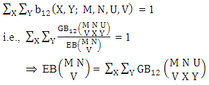 | (3.16) |
The both way B distribution is also known as the joint probability distribution of X and Y.Example 3.8: Let the bivariate probability distribution of example 3.4 find both way B distribution of (i) P(X = 0, Y = 4) and (ii) P(X = 4 , Y = 3).Solution: From the given table we get (i) P(X = 0, Y= 4) = 0.001 and (ii) P(X = 4, Y = 3) = 0.008.Definition 3.9 First way SB distribution: Let the joint distribution of two random variables X and Y is given then the first way SB distribution can be written as | (3.17) |
Remark: It should be noted that 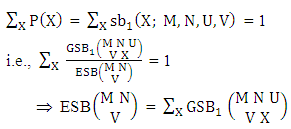 | (3.18) |
Example 3.9: Consider the GSB experiment  . Find the probability of getting (i) X = 1 and (ii) X = 2.Solution: We get the probabilities as
  Definition 3.10 Second way SB distribution: Let the joint distribution of two random variables X and Y is given then the second way SB distribution can be written as
 | (3.19) |
Remark: It should be noted that 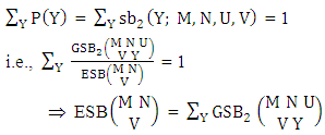 | (3.20) |
Example 3.10: Consider the GSB experiment  . Find the probability of getting (i) Y = 1 and (ii) Y = 3.Solution: We get the probabilities as
  Definition 3.11 Both way SB distribution: A two dimensional random variable (X, Y) is said to follow both way SB distribution if it assumes only non-negative values and its joint probability mass function is given by
 | (3.21) |
Remark: It should be noted that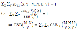 | (3.22) |
Example 3.11: Consider the GSB experiment  . Find the probability of getting (i) X = 0, Y = 2 and (ii) X = 3, Y = 3.Solution: We get the probabilities as
  Definition 3.12 First way AB distribution: Let the joint distribution of two random variables X and Y is given then the first way AB distribution can be written as
 | (3.23) |
Remark: It should be noted that 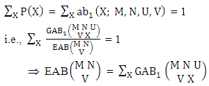 | (3.24) |
Example 3.12: Consider the GAB experiment  . Find the probability of getting (i) X = 1 and (ii) X = 3.Solution: We get the probabilities as
  Definition 3.13 Second way AB distribution: Let the joint distribution of two random variables X and Y is given then the second way AB distribution can be written as
 | (3.25) |
Remark: It should be noted that 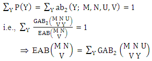 | (3.26) |
Example 3.13: Consider the GAB experiment  . Find the probability of getting (i) Y = 2 and (ii) Y = 3.Solution: We get the probabilities as
 Definition 3.14 Both way AB distribution: A two dimensional random variable (X, Y) is said to follow both way AB distribution if it assumes only non-negative values and its joint probability mass function is given by
 | (3.27) |
Remark: It should be noted that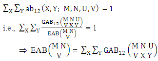 | (3.28) |
Example 3.14: Consider the GAB experiment  . Find the probability of getting (i) X = 1, Y = 2 and (ii) X = 3, Y = 3.Solution: We get the probabilities as
  Definition 3.15 First way SAB distribution: Let the joint distribution of two random variables X and Y is given then the first way SAB distribution can be written as
 | (3.29) |
Remark: It should be noted that 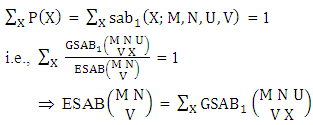 | (3.30) |
Example 3.15: Consider the GSAB experiment  . Find the probability of getting (i) X ≥ 2 and (ii) X ≤ 1.Solution: The table of example 27.3.4 represents bivatrate probability distribution of the experiment
  . Now we get from the table (i) P(X ≥ 2) = P(X = 2) + P(X = 3) + P(X = 4) = 0.514 + 0.228 + 0.015 = 0.757(ii) P(X ≤ 1) = P(X = 0) + P(X = 1) = 0.015 + 0.228 = 0.243.Definition 3.16 Second way SAB distribution: Let the joint distribution of two random variables X and Y is given then the second way SAB distribution can be written as
  | (3.31) |
Remark: It should be noted that 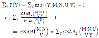 | (3.32) |
Example 3.16: Consider the GSAB experiment  . Find the probability of (i) Y = 3 and (ii) Y ≤ 3.Solution: The table of example 27.3.4 represents bi-variate probability distribution of the experiment
  . Now we get from the table (i) P (Y = 3 ) = 0.534(ii) P (Y ≤ 3) = P(Y = 2) + P(Y = 3) = 0.400 + 0.534 = 0.934.Definition 3.17 Both way SAB distribution: A two dimensional random variable (X, Y) is said to follow both way SAB distribution if it assumes only non- negative values and its joint probability mass function is given by
 | (3.33) |
Remark: It should be noted that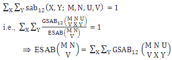 | (3.34) |
Example 3.17: Consider the GSAB experiment  . Find the probability of getting (i) X = 1, Y = 3 and (ii) X = 2, Y = 2.Solution: The table of example 27.3.4 represents bi-variate probability distribution of the experiment
  . Now we get from the table (i) P(X = 1, Y = 3) = 0.122(ii) P(X = 2, Y = 2) = 0.206.Definition 3.18 First way ASB distribution: Let the joint distribution of two random variables X and Y is given then the first way ASB distribution can be written as
 | (3.35) |
Remark: It should be noted that 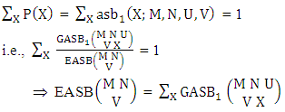 | (3.36) |
Example 3.18: Consider the GASB experiment  . Find the probability of getting (i) X = 0 and (ii) X = 3. Solution: The table of example 27.3.5 represents bi-variate probability distribution of the experiment
  . Now we get from the table(i) P(X = 0) = 0.031 (ii) P(X = 3) = 0.158.Definition 3.19 Second way ASB distribution: Let the joint distribution of two random variables X and Y is given then the second way ASB distribution can be written as
 | (3.37) |
Remark: It should be noted that 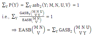 | (3.38) |
Example 3.19: Consider the GASB experiment  . Find the probability of getting (i) Y = 2 and (ii) Y ≤ 2.Solution: The table of example 27.3.5 represents bi-vatrate probability distribution of the experiment
  . Now we get from the table (i) P(Y = 2) = 0.571(ii) P(Y ≤ 2) = P(Y = 1) + P(Y = 2) = 0.143 + 0.571= 0.714.Definition 3.20 Both way ASB distribution: A two dimensional random variable (X, Y) is said to follow both way ASB distribution if it assumes only non negative values and its joint probability mass function is given by
 | (3.39) |
Remark: It should be noted that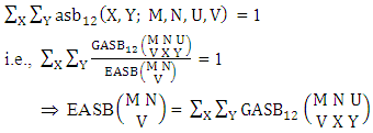 | (3.40) |
Example 3.20: Consider the GASB experiment  . Find the probability of getting (i) X = 0, Y = 2 and (ii) X = 2, Y = 3.Solution: The table of example 27.3.5 represents bi-variate probability distribution of the experiment
  . Now we get from the table (i) P(X = 0, Y = 2) = 0.018(ii) P(X = 2, Y = 3) = 0.146.
3. Applications
From the definitions stated in this paper we can find various joint probability functions, marginal probability functions and conditional probability functions.
4. Main Results at a Glance
The following is a list of probability laws developed in this paper.
5. Glossary
6. Conclusions
The paper finds an attractive Biswas distribution and related distributions. We get various joint probability functions, marginal probability functions and conditional probability functions from Biswas distribution. Combination distribution, permutation distribution, formation distribution and homogenation distribution are also found here.
References
| [1] | Deapon Biswas, Paper 4, B space, Bystematics My Classic, 2010 Self published, Chittagong, 2016 Monon Prokashon, Chittagong, Bystematics Vol. I and II, My Classic, 2018 Scholar’s Press EU, ISBN: 987- 620-2-30664-5 and 987- 620-2-30960-8. |
| [2] | Deapon Biswas, Paper 13, On the combinations, Bystematics My Classic, 2010 Self published, Chittagong, 2016 Monon Prokashon, Chittagong, Bystematics Vol. I and II, My Classic, 2018 Scholar’s Press EU, ISBN: 987- 620-2-30664-5 and 987- 620-2-30960-8. |
| [3] | Deapon Biswas, Paper 16, On the permutations, Bystematics My Classic, 2010 Self published, Chittagong, 2016 Monon Prokashon, Chittagong, Bystematics Vol. I and II, My Classic, 2018 Scholar’s Press EU, ISBN: 987- 620-2-30664-5 and 987- 620-2-30960-8. |
| [4] | Deapon Biswas, Paper 18, Fomrations, Bystematics My Classic, 2010 Self published, Chittagong, 2016 Monon Prokashon, Chittagong, Bystematics Vol. I and II, My Classic, 2018 Scholar’s Press EU, ISBN: 987- 620-2-30664-5 and 987- 620-2-30960-8. |
| [5] | Deapon Biswas, Paper 20, Homogenations, Bystematics My Classic, 2010 Self published, Chittagong, 2016 Monon Prokashon, Chittagong, Bystematics Vol. I and II, My Classic, 2018 Scholar’s Press EU, ISBN: 987- 620-2-30664-5 and 987- 620-2-30960-8. |
| [6] | Deapon Biswas, Paper 23, EB members, Bystematics My Classic, 2010 Self published, Chittagong, 2016 Monon Prokashon, Chittagong, Bystematics Vol. I and II, My Classic, 2018 Scholar’s Press EU, ISBN: 987- 620-2-30664-5 and 987- 620-2-30960-8. |
| [7] | Deapon Biswas, Paper 24, IB members, Bystematics My Classic, 2010 Self published, Chittagong, 2016 Monon Prokashon, Chittagong, Bystematics Vol. I and II, My Classic, 2018 Scholar’s Press EU, ISBN: 987- 620-2-30664-5 and 987- 620-2-30960-8. |
| [8] | Deapon Biswas, Paper 25, CB members, Bystematics My Classic, 2010 Self published, Chittagong, 2016 Monon Prokashon, Chittagong, Bystematics Vol. I and II, My Classic, 2018 Scholar’s Press EU, ISBN: 987- 620-2-30664-5 and 987- 620-2-30960-8. |
| [9] | Deapon Biswas, Paper 26, GB members, Bystematics My Classic, 2010 Self published, Chittagong, 2016 Monon Prokashon, Chittagong, Bystematics Vol. I and II, My Classic, 2018 Scholar’s Press EU, ISBN: 987- 620-2-30664-5 and 987- 620-2-30960-8. |


 find P(X = 2, Y = 1) where the experiment is first way arranged and second way selected.Solution: We know
  Definition 3.2 SB distribution: A two dimensional random variable (X, Y) is said to follow SB distribution if it assumes only non-negative values and its joint probability mass function is given by

 find (i) P(X =2, Y=3) and (ii) P(X=3,Y=1).Solution: We get
 Definition 3.3 AB distribution: A two dimensional random variable (X, Y) is said to follow AB distribution if it assumes only non-negative values and its joint probability mass function is given by

 find (i) P(X=1,Y=3) and (ii) P(X=2,Y=2).Solution: We get
 Definition 3.4 SAB distribution: A two dimensional random variable (X, Y) is said to follow SAB distribution if it assumes only non-negative values and its joint probability mass function is given by

 .
. Find the probability of getting (i) X = 0, Y = 2, (ii) X = 2, Y = 3 and (iii) Y = 4.Solution:
 We get from the above table(i) Probability of getting X = 0, Y = 2 i.e., P(X = 0, Y = 2) = 0.06(ii) Probability of getting X = 2, Y = 3 i.e., P(X = 2, Y = 3) = 0.274 (iii) Probability of getting Y = 4 i.e., P(Y = 4) = 0.066.Definition 3.5 ASB distribution: A two dimensional random variable (X, Y) is said to follow ASB distribution if it assumes only non-negative values and its joint probability mass function is given by

 .
. Find (i) P(X ≥ 2), (ii) P(X = 0, Y = 3), (iii) P(X ≤ 2, Y = 2) and (iv) P(X = 3, Y ≥ 2).Solution:
 Solution: We get from the above table (i) P(X ≥ 2) = P(X = 2) + P(X = 3) = 0.510 + 0.158 = 0.668(ii) P(X = 0, Y = 3) = 0.009(iii) P(X ≤ 2, Y = 2) = P(X = 0, Y = 2) + P(X = 1, Y = 2) + P(X= 2, Y= 2) = 0.018 + 0.172 + 0.291 = 0.481 (iv) P(X = 3, Y ≥ 2) = P(X = 3, Y = 2) + P(X = 3, Y = 3) = 0.090 + 0.045= 0.135Now we describe three kinds of B distributions i.e., first way B distribution, second way B distribution and both way B distribution and their different forms. Definition 3.6 First way B distribution: Let the joint distribution of two random variables X and Y is given then the first way B distribution can be written as


 . Find the probability of getting (i) X = 1 and (ii) X = 2.Solution: We get the probabilities as
  Definition 3.10 Second way SB distribution: Let the joint distribution of two random variables X and Y is given then the second way SB distribution can be written as

 . Find the probability of getting (i) Y = 1 and (ii) Y = 3.Solution: We get the probabilities as
  Definition 3.11 Both way SB distribution: A two dimensional random variable (X, Y) is said to follow both way SB distribution if it assumes only non-negative values and its joint probability mass function is given by

 . Find the probability of getting (i) X = 0, Y = 2 and (ii) X = 3, Y = 3.Solution: We get the probabilities as
  Definition 3.12 First way AB distribution: Let the joint distribution of two random variables X and Y is given then the first way AB distribution can be written as

 . Find the probability of getting (i) X = 1 and (ii) X = 3.Solution: We get the probabilities as
  Definition 3.13 Second way AB distribution: Let the joint distribution of two random variables X and Y is given then the second way AB distribution can be written as

 . Find the probability of getting (i) Y = 2 and (ii) Y = 3.Solution: We get the probabilities as
 Definition 3.14 Both way AB distribution: A two dimensional random variable (X, Y) is said to follow both way AB distribution if it assumes only non-negative values and its joint probability mass function is given by

 . Find the probability of getting (i) X = 1, Y = 2 and (ii) X = 3, Y = 3.Solution: We get the probabilities as
  Definition 3.15 First way SAB distribution: Let the joint distribution of two random variables X and Y is given then the first way SAB distribution can be written as

 . Find the probability of getting (i) X ≥ 2 and (ii) X ≤ 1.Solution: The table of example 27.3.4 represents bivatrate probability distribution of the experiment
  . Now we get from the table (i) P(X ≥ 2) = P(X = 2) + P(X = 3) + P(X = 4) = 0.514 + 0.228 + 0.015 = 0.757(ii) P(X ≤ 1) = P(X = 0) + P(X = 1) = 0.015 + 0.228 = 0.243.Definition 3.16 Second way SAB distribution: Let the joint distribution of two random variables X and Y is given then the second way SAB distribution can be written as

 . Find the probability of (i) Y = 3 and (ii) Y ≤ 3.Solution: The table of example 27.3.4 represents bi-variate probability distribution of the experiment
  . Now we get from the table (i) P (Y = 3 ) = 0.534(ii) P (Y ≤ 3) = P(Y = 2) + P(Y = 3) = 0.400 + 0.534 = 0.934.Definition 3.17 Both way SAB distribution: A two dimensional random variable (X, Y) is said to follow both way SAB distribution if it assumes only non- negative values and its joint probability mass function is given by

 . Find the probability of getting (i) X = 1, Y = 3 and (ii) X = 2, Y = 2.Solution: The table of example 27.3.4 represents bi-variate probability distribution of the experiment
  . Now we get from the table (i) P(X = 1, Y = 3) = 0.122(ii) P(X = 2, Y = 2) = 0.206.Definition 3.18 First way ASB distribution: Let the joint distribution of two random variables X and Y is given then the first way ASB distribution can be written as

 . Find the probability of getting (i) X = 0 and (ii) X = 3. Solution: The table of example 27.3.5 represents bi-variate probability distribution of the experiment
  . Now we get from the table(i) P(X = 0) = 0.031 (ii) P(X = 3) = 0.158.Definition 3.19 Second way ASB distribution: Let the joint distribution of two random variables X and Y is given then the second way ASB distribution can be written as

 . Find the probability of getting (i) Y = 2 and (ii) Y ≤ 2.Solution: The table of example 27.3.5 represents bi-vatrate probability distribution of the experiment
  . Now we get from the table (i) P(Y = 2) = 0.571(ii) P(Y ≤ 2) = P(Y = 1) + P(Y = 2) = 0.143 + 0.571= 0.714.Definition 3.20 Both way ASB distribution: A two dimensional random variable (X, Y) is said to follow both way ASB distribution if it assumes only non negative values and its joint probability mass function is given by

 . Find the probability of getting (i) X = 0, Y = 2 and (ii) X = 2, Y = 3.Solution: The table of example 27.3.5 represents bi-variate probability distribution of the experiment
  . Now we get from the table (i) P(X = 0, Y = 2) = 0.018(ii) P(X = 2, Y = 3) = 0.146.

 Abstract
 Reference
 Full-Text PDF
 Full-text HTML